Consider the two variable linear model
2.1: ![]()
Synonyms for y.
Synonyms for x.
In what sense is the equation linear?
How do we interpret ![]() ?
?
Suppose y represents the yield of bushels of corn per acre and x represents the amount of fertilizer applied per acre. What are the specific interpretations of ![]() ?
?
Suppose y represents compensation and x represents years of education. Now how do we interpret the coefficients?
2.5 Unconditional mean of the disturbance: E(u).
2.6 The conditional mean of the error: E(u|x).
Implication of 2.5 and 2.6: Suppose y represents compensation and x represents years of education in the model 2.1. We know that in addition to education one's compensation depends on ability. Note that ability is not on the RHS of 2.1, therefore its effect on education must be captured by the error term. The implication of this is that E(ability|education) should be constant across all levels of education, otherwise the result would be a violation of 2.5 - 2.6. Is E(ability|education) = k plausible?
![]()
Diagram
Two assumptions about the model
E(u) = 0
Cov(u,x) = E(ux) = 0
Now substitute away from u in the two assumptions to get
![]()
![]()
Using the principle of analogies, let's construct the sample analog to these assumptions about the population model.
 (2.14)
 (2.15)
Note that this analogy approach is tantamount to the method of moments since the parameters of interest will turn out to be functions of the moments of the underlying random variable y. Place hats on top of the betas to indicate that we want to chose these values for these unknowns so that the equalities hold. Solving (2.14) for the intercept in terms of the other expressions yields
![]() (2.17)
(2.17)
Take (2.17), put it into (2.15) and solve for our best guess for the unknown slope parameter.
![]() (2.19)
(2.19)
Equation (2.17) tells us that the sample regression line must go through the point of means in a graph of the function.
Equation (2.19) tells us that the slope is the ratio of the covariance between the independent and dependent variables to the variance of the independent variable.
Graph showing population regression function {E(Y|X=x)}, the sample regression line, observed values, fitted values and residuals.
Your text uses a data file called CEOSAL1 to illustrate this discussion. Go here for that data. The scatter with the sample regression line, in red, is pictured below:
 |
 |
All the data |
Just 15 observations |
Just to be sure that I agree with the author of the book I have included output from EVIEWS.
Dependent Variable: SALARY |
|
|
||
Method: Least Squares |
|
|
||
Date: 02/09/11 Time: 08:34 |
|
|
||
Sample: 1 209 |
|
|
|
|
Included observations: 209 |
|
|
||
|
|
|
|
|
Variable |
Coefficient |
Std. Error |
t-Statistic |
Prob. |
C |
963.1913 |
213.2403 |
4.516930 |
0.0000 |
ROE |
18.50119 |
11.12325 |
1.663290 |
0.0978 |
|
|
|
|
|
R-squared |
0.013189 |
Mean dependent var |
1281.120 |
|
Adjusted R-squared |
0.008421 |
S.D. dependent var |
1372.345 |
|
S.E. of regression |
1366.555 |
Akaike info criterion |
17.28750 |
|
Sum squared resid |
3.87E+08 |
Schwarz criterion |
17.31948 |
|
Log likelihood |
-1804.543 |
Hannan-Quinn criter. |
17.30043 |
|
F-statistic |
2.766532 |
Durbin-Watson stat |
2.104990 |
|
Prob(F-statistic) |
0.097768 |
|
|
|
|
|
|
|
|
|
|
|
|
|
The residual
First, a couple of definitions courtesy of some algebra:
![]()
![]()
![]() (2.30) The sum of the residuals is zero by assumption and construction; see (2.14)
(2.30) The sum of the residuals is zero by assumption and construction; see (2.14)
![]() (2.31) The correlations is zero by assumption and construction; see (2.15)
(2.31) The correlations is zero by assumption and construction; see (2.15)
Sums of Squares
 Total sum of squares: Note that this is the numerator of the sample variance of y. Another interpretation is that our best guess for y is to use the sample mean if we are prepared to disregard what we know about the relationship between x and y.
 Explained sum of squares: Note that this is the numerator of the sample variance of the fitted values for y.
 Residual sum of squares. This is the amount of variation in y that is left over after we account for the association between x and y. It is the variation in y that is NOT explained by our model.
SST = SSE + SSR The variation in y must be accounted for by the part that we can explain and that which we cannot.
How good is our model? If we are considering two different specifications, or models, which should we choose?
The coefficient of determination
R2 = SSE/SST The ratio of explained sum of squares to the total sum of squares.
R2 = 1 - SSR/SST This representation comes from a little algebraic manipulation. If the model could explain y perfectly then the coefficient of determination ought to be 1. It seems reasonable then to subtract the fraction of the variation in y that we can't explain in order to find the coefficient of determination.
So far we have discussed only models with a single explanatory variable on the RHS of the regression function. Looking at SSE and giving it a little thought suggests that one can make it bigger by including more explanatory variables, even if they don't have much to do with explaining y. The consequence of this is that one can always increase the coefficient of determination by including more variables. Later in the semester will talk about penalizing the R2 for including variables indiscriminately.
Centigrade versus Fahrenheit; inches or feet or yards? Linear or log?
Measurement
1. Change the scale of only the dependent variable by the constant k:
![]()
Just multiply the original coefficient estimate by the constant.
2. Change the explanatory variable by a multiplicative constant, but leave the dependent variable alone. If you multiply the observations on x by k, then the slope coefficient must change by the multiple (1/k). There is no impact on the intercept.
3. Suppose you add a constant to every observation on the dependent variable. What will be the impact on intercept and slope?
4. Suppose you add a constant to each observation on the independent variable. What will be the impact on the intercept and slope?
Functional Form
As long as we preserve the linearity in the unknowns we can still use OLS. The computer isn't so smart after all.
Level - level -- A straight line
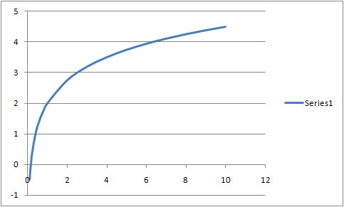
Level - log -- A 1% change in x produces how big a change in y? Depending on the sign of the slope coefficient this produces either a concave or convex line.
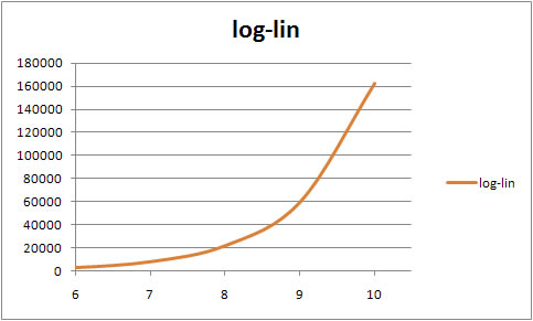
Log - Level
log - log -- A constant elasticity model
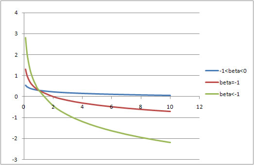
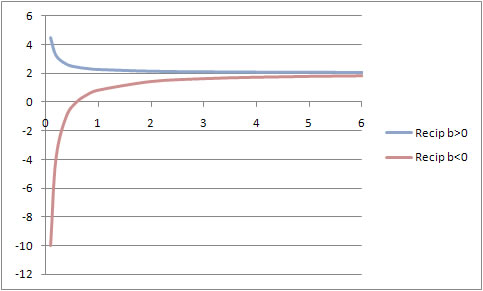
Level - reciprocal: y = bzero + b(1/x) and y = bzero - b(1/x)
Can you fill in the table below?
| Model Name | Symbolic Model | Interpretation of slope | Marginal Effect (dY/dX) | Elasticity (X/Y)(dY/dX) |
| Level - Level |
|
|
|
|
| Level - Log |
|
|
|
|
| Log - Level |
|
|
|
|
| Log - Log |
|
|
|
|
| Level - Reciprocal |
|
|
|
|
| Quadratic |
|
|
|
|
| Level-Interaction |
|
|
|
|
| Log-Reciprocal |
|
|
|
|
| Log-quadratic |
|
|
|
|
| Logistic |
|
|
|
Our model of the process that generated the data is
![]()
in which the intercept and slope are unknown and u is an unobservable random variable. With each sample we are able to estimate the slope and intercept and we get a set of least squares residuals that serve as "guesses" for the unobservable values taken by u.
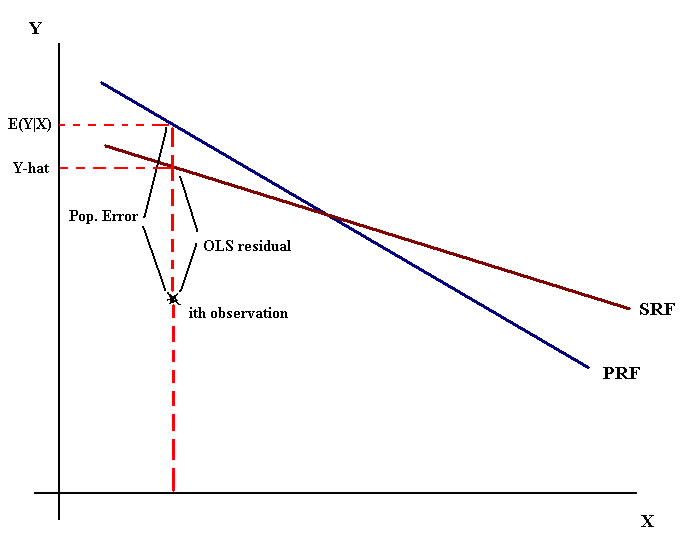
The OLS residual is computed from the data. The researcher never sees or observes the population error since the population regression function is unknown to the researcher. Nevertheless, there is a connection between the error, u, and the least squares residual. A bit of reflection on equation (2.1) and the graph leads us to write
![]()
And then substitute away from the actual and fitted values for y:
![]()
![]()
From this you can see two things: First, the least squares residual is never exactly equal to the error; the difference between the two is sample dependent. Second, on average the least squares residual is equal to the error, and is in turn equal to zero on average.
To estimate the population error variance we work by analogy once again. We would like the error variance to be independent of any particular realization of xi. That is,
![]() for all i.
for all i.
By analogy we would then use
But note that in this computation we will have used the data twice in constructing the OLS residual series. Therefore, while it qualifies as an estimator, there ought to be a penalty for previously using the data to estimate the slope and intercept. The revised estimator is then
The subscript LS, which stands for least squares, is added to distinguish it from what we first proposed. As it happens, the estimator we first proposed is the maximum likelihood estimator of the error variance.
The intercept and slope estimators are both unbiased. They are also consistent.
The LS error variance estimator is unbiased and consistent.
![]()
The standard errors of the estimators are just the square roots of these variances