Chapter 3

Multiple Regression

Motivation for Multiple Regression

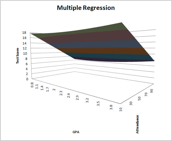
Simple regression is just a line or curve in a plane. Multiple regression gives us the opportunity to produce a surface in a multi-dimensional space. Having more than one explanatory variable allows us to explore all the richness of the phenomenon that interests us. When there are two regressors we might get something like

Interpreting coefficients

1. The coefficient is the marginal or partial effect of x₂ on y, all other variables held constant. By marginal effect we mean that a one unit increase in x₂ causes y to increase by the amount . The coefficient is also the partial derivative of y with respect to x₂. This is generalizable to many right hand side variables.

2. There is also an analogy to the total differential of calculus. Namely, in which we change all of the explanatory variables simultaneously.

3. A bit of algebra can be used to show that there is a correspondence between the regression coefficients and the partial correlation between x_i and y. By partial correlation we mean that we use all the RHS variables except x_i to explain y and then go on to see if there is any variation in y that is left over for x_i to explain.

Deriving the Least Squares Estimators

There are two approaches which turn out to be equivalent.

1. We could use our principal of analogy as we did for simple regression. For example,

These three equations could be solved for the three unknowns.

2. The second approach is to pick our guesses as to minimize the sum of squared differences between the observed values of y and our best guesses expressed as

.

2.a. If we are willing to assume that the specified model is correct then we can interpret the OLS estimator as a minimum distance estimator since the sum of squares is a distance measure.

2.b. The sum of squared errors is a quadratic form in the unknowns, therefore it will have a unique minimum that can be found by setting the first derivatives to zero and solving the resulting system for the unknowns. The objective function is

Sums of Squares and Goodness of Fit

All the sums of squares retain their previous definitions.

Similarly, R² is still SSE/SST or 1 - SSR/SST.

Properties of the Estimators

Assumptions

1. The model is presumed to be correctly specified.

2. We have a random sample of data for each of the random variables.

3. None of the independent variables is constant.

4. The independent variables are linearly independent of one another. The indepedent variables are said to be NOT collinear. Notice that in the same sentence we have used "independent" in two different ways.

5. As in the previous chapter the expected value of the error conditional on any of the independent variables is zero.

Theorem:

1. The OLS estimator is unbiased.
2. The OLS estimator is consistent.
3. In the class of linear unbiased estimators the OLS estimator has the smallest possible variance.

Inclusion of Irrelevant Variables

If an irrelevant variable is included in a model specification then logic tells us that the coefficient on that variable should be zero in the population regression function, and in any sample regression the estimate should be close to zero. Of course, in any given sample the coefficient on the irrelevant variable my not be close to zero either numerically or statistically.

Ommission of Relevant Variables

The ommission of a relevant variable is a problem.

The correct model is

but we mistakenly estimate the parameters of

In the mistaken model the slope estimator is given by

Now subsitute away from y by the correct model.

From the properties of the weights w_i we can write

The middle term is times the result of regressing x₂ on x₁ and the third term is zero in expectation. The direction of the bias depends on the sign of and the sign of the correlation between x₁ and x₂. If x₁ and x₂ are uncorrelated then, in the parlance of mathematics, they are orthogonal to one another and there is no bias.

Variances of the OLS slope estimators:

The sample correlation between x₁ and x₂ rears its ugly head when we consider the sampling variances of the slope estimators. This is important because we use the variances of the slope estimators in the denominator in the construction of the t-statistics for tests of hypothesis. If x₁ and x₂ are correlated then it could cause us to either under- or over-state the t-statistics.

Some definitions:

is the coefficient of determination for the regression of x_j on all of the other independent variables.

is the total sum of squares for x_j in the sample.

With some tedious algebra

What do we conclude?

A great big caveat is that under the assumptions of the previous chapter, multicollinearity is a problem in the particular sample. The only real solution is to get either more data or new data.