Inference in Regression Analysis

Sampling Distributions of the LS Estimators

1. Our starting point usually is to make the assertion that the correct model is

.

2. In addition to the assumptions about independence, we often say : The error is normally distributed with zero mean and finite variance.

3. Combining the pieces leads us to the conclusion that .

4. In earlier encounters we learned about the distributions of linear combinations of random variables with known distributions. For example, we learned that if X is a random variable with a normal distribution then the sample mean has a normal distribution, i.e., .

5. When the simple regression model was introduced we showed that the slope estimator could be written as . In this representation we see that the least squares estimator is a linear combination of random variables that are themselves normally distributed. All of this leads to the following big idea:

Student's t-test for a slope

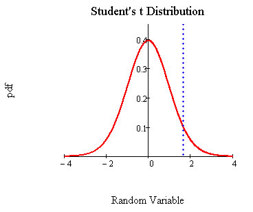
The "critical" t-statistics that we take out of the tables and against which we compare our observed t-statistic will depend on the level of the test, the degrees of freedom and whether the test is one tail or two.

What is the p-value for a t test?

Statistical significance versus practical significance?

An Example Using EVIEWS

Using a dataset on salaries of players in US major league, Paul Murkey of Murky Research, Inc estimated the coefficients of the following model

.

We'll refer to this as the maintained model, or Big Omega.

The variable legend is

• salary - player salary
• years - years in M:LB
• gamesyr - average games played per year
• bavg - player's lifetime batting average
• hrunsyr - player's average number of home runs per year
• rbisyr - players's average number of runs batted in per year

The empirical results for Big Omega are in the following table:

Big Omega: The maintained model

The estimate of the coefficient on bavg is 0.000979 and the standard error of the estimate is 0.001104. The observed "t" test statistic for testing the null hypothesis that the bavg coefficient is zero against the alternate that it is not zero is 0.886802 . The degrees of freedom for the test would be 353-6 = 347. If the level of the test is, say, 10% then we would look up the critical t for 347 degrees of freedom that cuts off 5% in each tail. The critical values are . Since the observed t-statistic falls between these two values we fail to reject the null hypothesis that the coefficient on bavg is zero.

Another equivalent way to conceptualize the test of hypothesis is to state it in terms of p-values. Refer again to the coefficient on bavg. We see t^obs = 0.8868. If the coefficient is indeed zero then the probability of seeing a t-statistic this large or larger is 0.37. Since the p-value is bigger than the chosen 5% per tail we again fail to reject the null.

Confidence Intervals

           [ , ]

Testing a Linear Combination of the Slopes

The model is

Suppose that our hypothesis is

The natural thing to do is to use to estimate . Hence we can make the substitution into the null and recognize that we have a linear combination of random variables. Therefore, we can use this intuition to use the generic form for the t-statistic and construct a t-statistic as:

The standard error is the square root of the variance of the linear combination. The following expression is a little more general than we need, so for the example we would set g=h=1 and just use the plus sign in the sum.

To illustrate this we'll again refer to the baseball example again. This time we'll test the null hypothesis that coefficients on hrunsyr and rbisyr are equal against the alternate that they are not. Formally this is stated as

To put it into the same form as that used at the start of this section and so that the construction of the t-statistic is more transparent we'll restate the null and alternate as

For the purposes of the example g = 1 and h = -1. Also, . Now we need to know the variances and covariances between the coefficient estimators. From EVIEWS the coefficient covariance matrix is:

                                                                    Coefficient Covariance Matrix

The variance for the hrunsyr coefficient is 0.000258. Note that you should be able to find the square root of this in the regression results table. The variance for the rbisyr coefficient is 0.0000515; again, you should be able to find the square root of this in the regression results table. The covariance between the hrunsyr and rbisyr coefficients is -0.000103.

Now use all the pieces to assemble the observed t-statistic for the linear combination of coefficients:

= 0.161

This is a very small observed t-statistic so we conclude that we do not reject the null.

Testing a Set of Linear Restrictions

Initially we believe that both durability as a player (years and gamesyr) and performance (bavg, hrunsyr and rbisyr) matter in the determination of one's salary. To see if there is any value to our belief we estimate the parameters of the following model:

                              (1)

This was what we referred to as Big Omaga up above. The result of the exercise is the following table:

In the tabulated results we see that for the performance variables the t-statistics are quite low and the corresponding p-values are quite large. To see if the performance varaibles as a group do not matter we specify an alternate model, referred to as Little Omaga:

                                                 (2)

Notice that this revised model is a nested alernative to the model with which we started. We'll refer to this restricted model as Little Omega.

The results for (2), Little Omega, are below:

Now our task is to decide whether the restrictions we imposed are 'wrong.'

In going from the Maintained Model, Big Omega, to the alternate model, Little Omega, we are implicitly testing the following formal hypothesis:

All three coefficients are zero against the alternate that on or more of them is not zero. This is a set of linear restrictions.

Another formula to know:

This is another generic test statistic.

In this formula df1 is the number of restrictions imposed in oder to get from Big Omega to Little Omega. df2 is the number of degrees of freedom in the error variance estimator for the Maintained Model: n-k-1. SSR has the usual meaning: sum of squared residuals. The subscripts, little omega and big omega, tell you which sum of squared residuals goes where.

Using it for our baseball example:

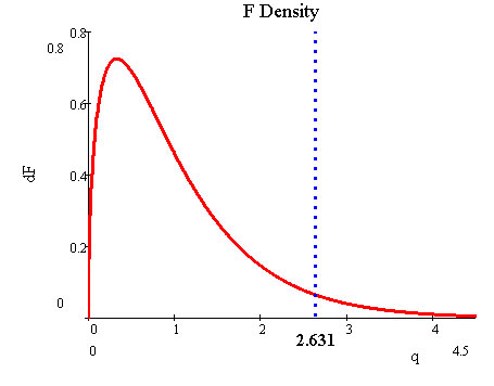
If we choose α = 0.05 then the critical F is 2.631.

Alternatively, the p-value,or probability in the upper tail, for our observed F is ~0.0

We reject the proposition that the performance varibles don't matter. The likelihood of getting an observed F as large as ours is extremely unlikely if performance variables don't matter.

A graph of the story is the following.