1. Definitions: Homoscedasticity versus heteroscedasticity
2. Did the variance of the error term play a role in proving the OLS estimator to be unbiased and consistent?
3. Does heteroscedasticity affect the coefficient of determination?
4. By the Gauss Markov Theorem we know that the OLS estimator is 'best' in the class of linear, unbiased estimators. What do we mean by best?
5. To prove the Gauss Markov Theorem the only essential assumptions were
If points 2. and 3. are true, then why sweat the presence of heteroscedasticity? Your answer should hinge on "We are in the business of testing hypotheses." The more precise our estimator, the more confident we are in our hypothesis test conclusions. When we talk about being precise, we are talking about statistical efficiency. Recall that the statistically efficient estimator is the one with the smallest variance in some specified class. Being precise depends on the variance of our estimator. The variance of the OLS estimator depends on the variance of the error term. The more we know about the variance of the error term, the more we know about the variance of our estimator.
To get the EVIEWS smoke work file that I used for the examples in this section of the outline just give a little click. To see how I created variables and did some other manipulations you might want to look at the commandlog.
For illustrative purposes we will use a simple regression model. The results and consequences outlined for the simple regression model can be scaled up to the multiple regression model with some algebra.
![]()
As before, we will assume that the error has zero mean.
![]()
This time we will be really audacious and daring and assume that the error variance differs from observation to observation.
![]()
For the simple regression model the OLS slope estimator was shown to be
![]()
Do you recall the definition of wi from an earlier chapter? With the assumption of zero mean for the error term, the LS estimator is still unbiased. The definition and derivation of the variance of the slope coefficient is
![]()
Can you outline verbally the steps and expectation rules subsumed in the second equality? Substituting away from the wi we can write
![]()
Then, applying the analogy principle that we have used to good effect in the past, we can use the squared least squares residuals as estimators for the observation dependent error variances. That is
![]()
As stated before, this is generalizable to the multiple regression case, but we'll leave it to the text and EVIEWS to figure out the details. We would use the square root of this variance estimator in the denominator of our usual t-statistic. To show the effect of correcting for heterscedasticity we'll consider a simple example.
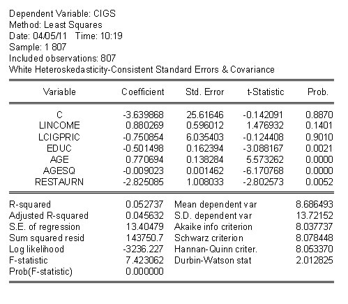
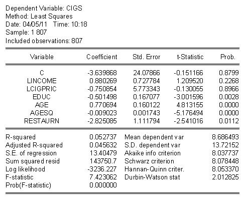
OLS Standard Errors No correction for heteroscedasticity |
Heteroscedasticity Robust Standard Errors Correction for heterscedasticity |
 |
|
Since we are in the business of testing hypotheses, we should start with a statement of the test of hypothesis. Namely,
![]()
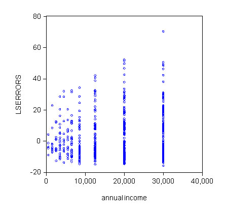
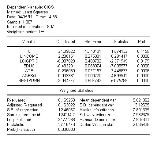
Often times the source of the heteroscedasticity is related to some exogenous variables that might even be the independent variables of the model. For example, in a model of corporate sales we would expect the variance of sales at large firms to be bigger than the variance of sales at small firms. In our cigarette example above, because nicotine and tar are understood to be addictive, we might expect greater variation in consumption among older people. In the tests for heteroscedasticity we exploit this potential for explaining heteroscedasticity.
Sometimes a plot of the residuals against the independent variables tells us a lot. In such a plot we expect the homoscedastic LS residuals to fall in a uniform band around zero regardless of the values taken by the explanatory variables. Consider this pair of graphs for the cigarette example.
 |
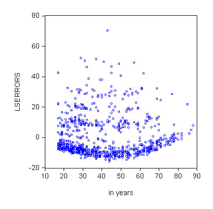 |
Either one of these scatter plots suggests that heteroscedasticity is a problem. As appealing as a simple eyeball test may be, we need to use a method that is a little more rigorous.
Recipe
1. Obtain the OLS residuals for the posited model.
2. Square each of the OLS residuals.
3. Estimate the coefficients in the model ![]()
4. Get the coefficient of determination from step three (3) and call it ![]() . In some places you will see this referred to as the uncentered coefficient of determination, but we won't go into the explanation other than to say that the mean of the residuals is zero so the regression in step (3) doesn't really need an intercept.
. In some places you will see this referred to as the uncentered coefficient of determination, but we won't go into the explanation other than to say that the mean of the residuals is zero so the regression in step (3) doesn't really need an intercept.
5. At this point we can use this residual based R2 in either one of two ways:
a.
This is the familiar F-statistic. The implied null is that coefficients estimated in step (3) are all zero, in which case the errors would be homoscedastic.
b.This is an asymptotic test statistic with the chi-square distribution. This is commonly known as the Breusch-Pagan test statistic.
For the cigarette example we have the result
 . The critical F at the 5% level is 2.616.
For the B-P test we get LM=800(0.039973) = 31.9874 . The critical chi-sq is 12.59.
In either case we reject the null hypothesis of homoscedasticity. Given the graphs that we saw, this is not an unexpected result.
We have to keep the legions of statisticians and econometricians busy. To this end Hal White came up with a variant of the Breusch-Pagan test. And to make matters more complicated there are two different recipes for the White test.
1. Obtain the OLS residuals for the posited model.
2. Square each of the OLS residuals.
3. Estimate the coefficients in the model that has as its LHS the squared OLS residuals. On the right hand side include all of the original RHS variables, their squares, and their cross products. Hence for a model with two RHS variables the auxiliary regression would look like ![]() .
.
4. Using the coefficient of determination for this model, construct the LM statistic.
For the cigarette example this recipe requires regression of the squared LS residuals on an intercept and twenty variables. That regression gives a chi-square test statistic = 786*0.059329 = 46.63. We know from the previous B-P test that this is a significant chi-square and we reject the null hypothesis.
1. Obtain the OLS residuals for the posited model.
2. Square each of the OLS residuals.
3. Estimate the coefficients in the model that has as its LHS the squared OLS residuals. On the right hand side we'll just include the fitted values and their square. Since the fitted values are linear combinations of all the exogenous variables this is roughly equivalent to the first recipe, but uses fewer degrees of freedom and involves less typing.
4. Using the coefficient of determination for this model, construct the LM statistic.
For the cigarette example this recipe yields LM = 804*0.032928 = 26.47, and again the null of homoscedasticity is rejected.
The cure is to rescale, or weight, the observations, and implicitly the error, so that the variance becomes constant. Once the variance is constant we can proceed as we normally would.
Recipe for Feasible GLS
1. Run the posited regression model and save the OLS residuals.
2. Square the residuals and take their log. Call the series "g".
3. Run a regression of "g" on the set of independent variables and obtain the fitted values, call them "ghat".
4. Construct h_hat = exp(ghat).
5. Go back to the original model and do weighted least squares using 1/h_hat as the weights.
For our cigarette example the regression results become
The world is neither flat nor getting smaller (notwithstanding the book by Thomas L. Friedman), nor is it linear. Apart from the question of omitting relevant variables there is the question of functional form. As you have come to expect, there is a test to see if you have proposed the correct functional form. Also, not surprisingly, there are several approaches.
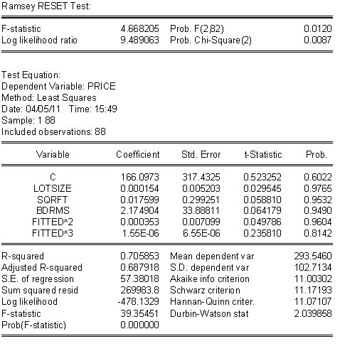
Ramsey's test is predicated on the idea that we should work with nested alternatives so that we can use the usual F-statistics.
Recipe
1. The null hypothesis is that your proposed model is correct. E.g. ![]()
2. The suspicion is that there might be some interaction, quadratic and cubed terms on the RHS that would add some curvature and twist to the plane posited in step (1). The rub is to account for this possibility without knowing exactly which RHS variables are involved and without eating up lots of degrees of freedom in the process of trying to uncover the non-linearity. Ramsey has suggested the use of an alternative model which serves this purpose and then testing the joint significance of the added terms. His trick is implemented as the specification of an auxiliary regression, e.g., ![]() . Note that this gets all the squared, cubed and interactions that you could construct, but at the cost of only two degrees of freedom.
. Note that this gets all the squared, cubed and interactions that you could construct, but at the cost of only two degrees of freedom.
3. Run OLS on the model in (1). Use the fitted values to construct their squared and cubed terms.
4. Run OLS on a revised model that includes the original variables plus the fitted squared and cubed dependent variable terms.
5. Construct an F-test on the joint significance of the squared and cubed fitted variable coefficients.
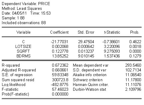
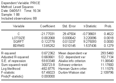
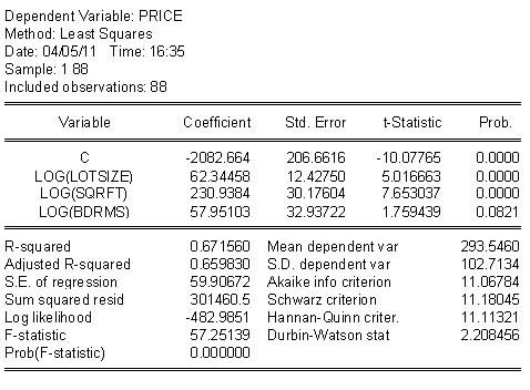
As an example, consider the housing price model in the table below. For cross section data the linear model on the right looks pretty good. In the table on the right there is ample evidence that the better model would include some nonlinearities.
 |
 |
Sometimes the competing non-linear models are not nested alternatives to one another. On the surface at least it appears as though we are stuck. Not to panic. As long as the variable to be explained is the same in the two models there is a work-around that is similar in spirit to Ramsey's approach.
You can get the EVIEWS file for this example with a little click.
Suppose that the competing models for home prices are
![]() (N01)
(N01)
![]() (N02)
(N02)
The idea is that if the linear model (N01) is fine then inserting the non-linear log terms will contribute nothing to the explanatory power of the model. Similarly, if linear terms do not belong in the semi-log model (N02) then adding them will not improve the explanatory power of the model. The procedure would be as follows:
Recipe
1. Fit both models to the data and save the fitted values of the dependent variable.
2. Name the fitted values ![]() , respectively for N01 and N02.
, respectively for N01 and N02.
3. Put ![]() in N02 and
in N02 and ![]() in N01 and run the regressions again.
in N01 and run the regressions again.
4. Do t-tests on the hat terms in the auxiliary regressions.
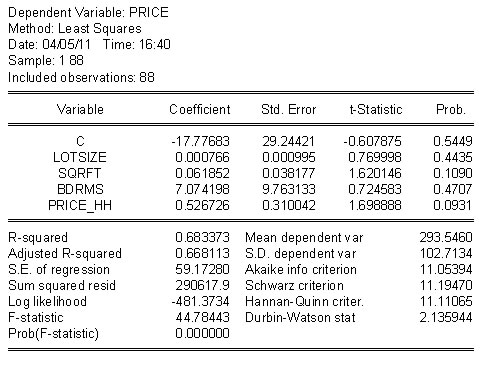
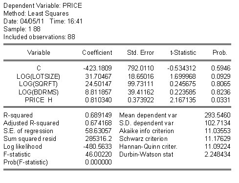
As an example consider the home price model again. In the top row both models seem to do pretty well: High R2 and significant coefficients. In the second row we have swapped fitted values of the dependent variables. In the linear model the addition of the non-linear term, first column of second row, improves the R2 a little, but the t-statistic is not significant for a two tail test. On the other hand, when we add the linear term to the semi-log model the t-statistic is significant at better than 10%, but notice that two of the slopes are not longer significant. HRH. how do we make sense of this?
 |
 |
 |
 |
In addition to education and experience we expect that ability is determinative of wages as well. How do you measure ability? Can you think of other examples of unobservables: How about teacher ability and performance and merit pay? In cases like these you can probably say "I know ability when I see it, but I don't know how to measure it."
Suppose that we have the model
![]()
in which ![]() is not observed, but we do have a proxy that can stand in for it. Call the proxy, or stand in, z. Its relationship to
is not observed, but we do have a proxy that can stand in for it. Call the proxy, or stand in, z. Its relationship to ![]() is as follows:
is as follows:
![]()
Since we don't observe ![]() it is proposed to use z instead. This will work as long as:
it is proposed to use z instead. This will work as long as:
When we plug and chug we end up estimating the coefficients of
![]()
Do we have enough equations in the unknowns to estimate all of the coefficients of the original model?
If we measure the dependent variable with error then our LS estimators are still unbiased. However, the error includes not just the population disturbance, but also the errors associate with the mistakes we make in measuring the dependent variable. What is the consequence of this for the precision with which we estimate the model coefficients?
Measuring the independent variable(s) with error is a whole 'nuther' kettle of fish. There are two cases to consider. For both we have a common starting point. The model is
![]()
where x1* is the household's actual income. However, it is commonplace in surveys for households to be deceitful in reporting their income. Instead of telling us that their income is x1*, they tell us that it is x1. The error that is made is random (every household tells a different size lie) and is given by
![]()
Case 1
Assume that Cov(e1,x1) = 0. The result is that the measurement error finds its way into the model error u with the consequence that the overall error variance is bigger and, for a given sample size, our t-statistics will be smaller. Other than less precise estimates of the unknown coefficients, the OLS estimators retain their usual properties: unbiased and consistent.
Case 2: Classical Errors in Variables
Now instead of Cov(e1,x1) = 0, we suppose that Cov(e1,x1*) = 0, which implies that e1 and x1 must be correlated.
![]()
To see what the consequence is for OLS let's do a bit of algebra: Begin by rearranging the measurement error.
![]()
Substitute into the original model
![]()
Rearrange
![]()
Now we can see the the revised model error is correlated with one of the RHS variables. Construct the OLS estinmator for the slope coefficient
![]()
The most important thing to note is that the numerator in the third term is the covariance between x1 and e1, which we know is not zero. It is in fact equal to Var(e1). Therefore OLS is no longer unbiased and is no longer consistent. The denominator of the third term is Var(x1*) + Var(e1). We can conclude that the third term is in the interval [-1, 0], so LS underestimates the true parameter. This is attenuation bias.
Data can be missing in several ways.
1. We may have missing observations on the RHS variables. There is little to be gained by trying to use extrapolation to fill in the missing observations.
2. The dependent variable may be truncated. Truncation means that we just don't have data for certain magnitudes of the dependent variable. For example, you have done a study of new car purchases for 2010. When you call on household j they say they would have liked to buy a new car but everything on the market exceeded their reservation price. The OLS estimators get reweighted by the part of the error distribution that we actually can see.
3. The dependent variable may be censored. An example of this is 'top coding.' In a survey respondents are asked their income. Their answer is coded in to intervals that are $10k wide starting with 0, unless they earn $100k or more, in which case they are coded as $100k. Now we know how many persons are in the last category, but we really have no idea what their income is. Again, OLS gets reweighted to account for the misshapen error distribution.
1. Exogenous sample selection based on RHS variables presents no problem.
2. Endogenous sample selection based on the dependent variable requires use of two stage estimators. In the first step we try to explain why an individual was chosen. In the second step estimate the parameters of the model of interest.
The principle of least squares uses squared errors in estimator construction. If an observaton lies far away from the rest of the sample then its associated error will be quite large, and squaring it makes it even bigger and more influential. To overcome such things scholars now use quantile regression and kernel regression.
Quantile regression has the added advantage that it allows us to estimate other parts of the distribution of the dependent variable beyond the conditional mean.
Kernel regression allows us to estimate non-linear, non-parametric functions of the data that are robust to all sorts of data problems.