As a further check I compared some of the individual
terms in the matrix to be inverted. Those I checked
differed only in the fourth or fifth decimal place.
As we know from the Mars lander, units and rounding
errors can make a great deal of difference.
5. Learning curve and
autocorrelation.
The data used to create the question are hidden in the
following region:
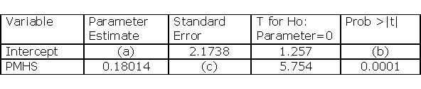
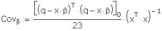
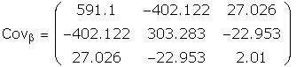
b. Compute the efficient estimator. Since I have the
original data I show the result using them.
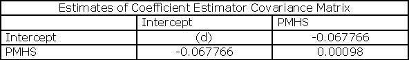
The coefficient covariance matrix is estimated to be:
Notice that the variances are smaller than when the
data is not corrected for heteroscedasticity.
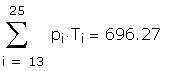
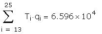
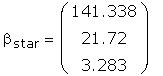
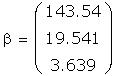
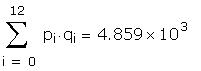
Computing the coefficient estimates using the sums of
squares and cross products as they were given to you
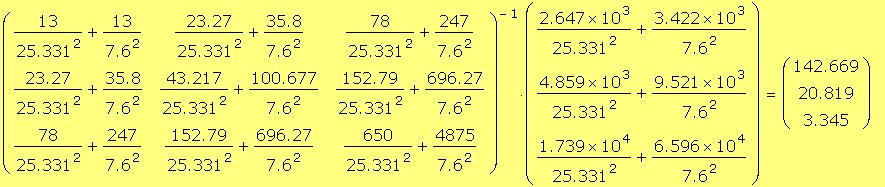
These estimates differ numerically from those using
the original data. This is do to rounding errors.
To convince you I have redone the same matrix calculations
using the symbolic sums of squares and cross products.
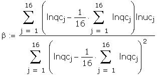
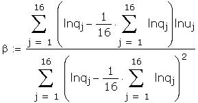
b. Compute an estimate
of r
the serial correlation coefficient.
c. 1971 production is expected to be 3800. What is
the point prediction for unit costs?
We have to restimate the model correcting for autocorrelation,
a. Compute the Durbin-Watson statistic and test for
autocorrelation at the 5% level
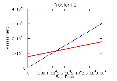
The blue line has slope 1. The red line is equation
1, with slope of .34. Below a sale price of about
$11,000 the ratio of assessment to sale price is greater
than 1, but it decreases for as home value in the market
grows. You can make a similar argument for equation
4.
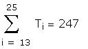
3. Australian wheat
growing
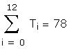
Set the sample size and a time index.
Create and intercept and a trend.
In MathCAD the data is hidden inside the area represented
by the horizontal line.
Create the design matrix.
Estimate the model parameters.
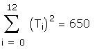
Create indices to split the sample, then create new
data sets for each half and estimate the coefficients.
Temple University
Department of Economics
Final Exam Key
Econ 615
Fall 2001
1.a. Show that the covariance of the RLS and OLS estimators
is equal to the variance of the RLS estimator.
Factor out the b
hat - b term
and make use of the fact that bhat - b
is equal to (x'x)-1x'u.
We have the definition of covariance Cov(bhat, b*
) = E(b
hat-b)(b*
-Eb*)'.
which is the desired result.
b. When testing the hypothesis
that bhat
- b
*=0 we would ordinarily need Var(bhat-b*)
= Var(bhat)+Var(
b
*)-2Cov(bhat,b
*). By the inequality proved in part a we only need
Var(bhat)-Var(
b
*). This makes construction of the Wald statistic much
simpler.
2. a
. (1) For each $1 increase in sale price the assessment
will be only $.34 higher. There is evidence of inequity.
This model and its interpretation is similar in spirit
to the marginal propensity to consume and average propensity
to consume debate in Keynesian economics. Specifically,
you ought to have discussed at least tangentially the
picture following part 2.c.
(2) For each $1 increase in sale price the ratio
of assessment to sale price will fall 4.57. We would
expect the coefficient to be zero if there was no inequity.
(3) The elasticity
of assessment with respect to sale price is .67. That
is a 1% increase in sale price will result in only
a .67% increase in assessment. So assessment rises
less than proportionately to an increase in sale price.
There is evidence of inequity
(4) For each $1increase in assessment, the sale
price will rise by $.77. Did you notice that the R2
is the same as equation 1. Do you know why? Also,
this model is equivalent to specifying model 1, but
instead of minimizing the errors in the A direction(or
vertical dimension) they errors are minimized in the
sale price direction (or horizontal dimension).
(5) for each $1 rise in assessment the ratio
of assessment to sale price will fall by .0000004.
So assessment as a fraction of home value is smaller
for more highly assessed homes. Notice that there
is no overall significance here. Why?
b.
The debate focuses on explaining variation in sales
price as a function of assessment, or assessment as
a proportion of sale price. There is also a question
of chronology and causality.
c.
(2) and (5) permit a non-linear relationship that
directly addresses the issue of assessment as a proportion
of sale price, whereas (1) and (4) do not.
The observed F falls in the rejection region.
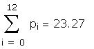
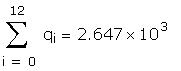
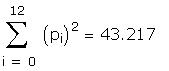
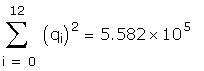
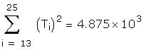
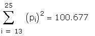
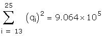
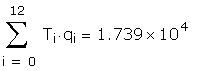
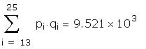
The sums of squares and cross products given in the
question were created here.
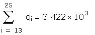
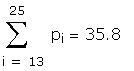
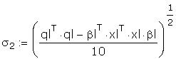
Estimate the standard deviation of the error term for
each half the sample. This information was given in
the question.
a. Test the hypothesis of homoscedasticity at the 5%
level.
The critical F with <10,10> degrees of freedom
is