Hwk 3: ANOVA and Simple OLS

Temple University
Department of Economics

Economics 615 Introduction to Analysis of Variance, Simple Regression
and Hypothesis Testing

1. (HT) In order to test whether four brands of gasoline give equal performance in terms of mileage, each of three cars was driven with each of the four brands of gasoline. Then each of the (3x4=12) possible combinations was repeated four times. The number of miles per gallon for each of the four repititions in each cell is recorded in the table below.

Brand of gasoline
Car	1		2		3		4
1	21.0	14.9	16.3	20.0	15.8	19.4	17.8	17.3
1	16.2	18.8	15.2	21.6	14.5	14.8	18.2	20.4
2	20.6	19.5	15.5	16.8	16.6	13.7	18.1	17.1
2	20.8	18.9	17.4	19.4	18.2	16.1	21.5	19.1
3	14.2	13.1	17.4	18.1	15.2	16.7	16.3	16.4
3	16.8	17.4	16.4	16.9	17.7	18.1	17.9	18.8

The possible model of gasoline consumption is

i=1,2,3 cars

j=1,2,3,4 brands of gas

andis the interaction between car and brand.

Test the following hypotheses:
a. The type of car does not matter.
b. The type of gasoline does not matter.
c. Neither the car nor the gasoline matters.
d. The interaction effect is zero.

Note that I added a few lines to the question above in order to provide alittle more clarity. Since you already have the data I won't reproduce it. In what follows I provide answers to the questions using both ANOVA and regression analysis. First comes the ANOVA output using EXCEL.

Anova: Two-Factor With Replication

SUMMARY	Gas 1	Gas 2	Gas 3	Gas 4	Total
Car 1
Count	4	4	4	4	16
Sum	70.9	73.1	64.5	73.7	282.2
Average	17.73	18.28	16.13	18.43	17.64
Variance	7.40	9.13	5.08	1.87	5.58

Car 2
Count	4	4	4	4	16
Sum	79.8	69.1	64.6	75.8	289.3
Average	19.95	17.28	16.15	18.95	18.08
Variance	0.82	2.64	3.47	3.56	4.40

Car 3
Count	4	4	4	4	16
Sum	61.5	68.8	67.7	69.4	267.4
Average	15.38	17.20	16.93	17.35	16.71
Variance	4.23	0.53	1.67	1.47	2.24

Total
Count	12	12	12	12
Sum	212.2	211	196.8	218.9
Average	17.68	17.58	16.40	18.24
Variance	7.20	3.61	2.94	2.36

ANOVA
Source of Variation	SS	df	MS	F	P-value	F crit
Car	15.61	2	7.80	2.24	0.12	3.26
Brand	21.58	3	7.19	2.06	0.12	2.87
Interaction	36.12	6	6.02	1.73	0.14	2.36
Within	125.53	36	3.49

Total	198.84	47

In the ANOVA table the row labeled 'Car' provides the information for the hypothesis that the type of car does not matter. The observed F is 224 and the critical F at 5% is 3.26, hence we cannot reject the null. The labeled 'Brand' has an observed F=2.06 against a critical F=2.87. Again, we cannot reject the null. To test the hypothesis that neither 'Car' nor 'Brand' matters we add together the two SS and divide by the total degrees of freedom, then divide that result by the 'within MS' to get an observed F=2.13. The 5% critical F for 5 and 36 degrees of freedom is F=2.49 (about). We cannot reject the null. From the table we also cannot reject the null hypothesis that there are no interaction effects.

Now for some OLS results: The first regression model has an intercept and dummies for 'type of car' and 'brand of gas". You will note that the 'Regression Sum of Squares (37.19) is equal to the sum of the 'Car' and 'Brand' SS in the table above.

SUMMARY OUTPUT

Regression Statistics
Multiple R	0.43
R Square	0.19
Adjusted R Square	0.09
Std Error	1.96
Observations	48

ANOVA
	df	SS	MS	F	Significance F
Regression	5	37.19	7.44	1.93	0.11
Residual	42	161.66	3.85
Total	47	198.84

	Coefficients	Standard Error	t Stat	P-value	Lower 95%	Upper 95%
Intercept	17.48	0.69	25.20	0.00	16.08	18.88
Car1	0.93	0.69	1.33	0.19	-0.47	2.32
Car 2	1.37	0.69	1.97	0.06	-0.03	2.77
B 1	-0.56	0.80	-0.70	0.49	-2.17	1.06
B2	-0.66	0.80	-0.82	0.42	-2.27	0.96
B3	-1.84	0.80	-2.30	0.03	-3.46	-0.23

SUMMARY OUTPUT		In the second regression model there are dummies for 'Car', 'Brand' and the interaction between the two, for a total of eleven dummies and one intercept. Now the Regression Sum of Squares is equal to the sum of SS for 'Car', 'Brand' and 'Interaction' in the original ANOVA table.

Regression Statistics
Multiple R	0.61
R Square	0.37
Adjusted R Square	0.18
Std Error	1.87
Observations	48

ANOVA
	df	SS	MS	F	Significance F
Regression	11	73.31	6.66	1.91	0.07
Residual	36	125.53	3.49
Total	47	198.84

	Coefficients	Standard Error	t Stat	P-value	Lower 95%	Upper 95%
Intercept	17.35	0.93	18.58	0.00	15.46	19.24
C1	1.08	1.32	0.81	0.42	-1.60	3.75
C2	1.60	1.32	1.21	0.23	-1.08	4.28
B1	-1.98	1.32	-1.50	0.14	-4.65	0.70
B2	-0.15	1.32	-0.11	0.91	-2.83	2.53
B3	-0.43	1.32	-0.32	0.75	-3.10	2.25
c1b1	1.28	1.87	0.68	0.50	-2.51	5.06
c1b2	0.00	1.87	0.00	1.00	-3.79	3.79
c1b3	-1.87	1.87	-1.00	0.32	-5.66	1.91
c2b1	2.98	1.87	1.59	0.12	-0.81	6.76
c2b2	-1.52	1.87	-0.82	0.42	-5.31	2.26
c2b3	-2.37	1.87	-1.27	0.21	-6.16	1.41

Using the regression sums of squares we can do the tests requested in parts c. and d. In order to do the test in parts a. and b. I would have to provide the results for two more regressions. Do you know what their specifications would be? What results, in terms of SS, would you expect to see?

Finally, note that none of the regression coefficients in either model are different from zero in a statistical sense.

The data in capm.txt is an ASCII text file. The first row has the variable names MARKET, RKFREE and Motor. Market is the market rate of return as a weighted monthly average of the NY and American Stock Exchanges for January 1978 through December 1987 (120 months). RKFREE is the return on 30-day U.S Treasury bills. It is understood to be the risk free rate. Motor is the monthly return for Motorola. By clicking you can retrieve a self-extracting file that contains this question set, the data, and a bit of MCD code which will read the data.
a. Plot the observations for the last thirty six months (all 120 observations wouldn't look like much).

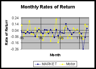
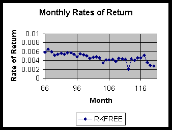
There is much more variation in the market rate and in the rate for Motorola than there is in the risk free rate.

Using the data construct Firm=Motor-RKFREE and MktIndex=Market-RKFREE. Compute the sample means for Motor, MARKET, RKFREE, Firm and MktIndex.

Average	0.007	0.008
Std Dev	0.069	0.090
	Mkt-RKF	Motor-RKF

Annualize the monthly returns.

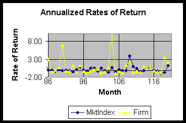
This done by applying Annual=(((1+Monthly)^12)-1) to the appropriate series.

d. Plot the annualized series for Firm and MktIndex for the last 36 months.

Discuss the two plots you did.

The second plot annualizes the monthly data {(((1+monthly r of r)^12)-1)} after subtracting out the return one could have earned by investing in a risk free bond.

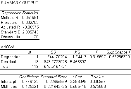
f. From the annualized data estimate the coefficients in the regression

Using the least squares residuals from this regression compute an estimate of the error variance.

Compute estimates of and .

From the regression output:

and

Test the hypothesis that the intercept is zero.

From the regression output the observed t is 3.38. This is significantly different from zero, so reject the null.

Test the hypothesis that the slope is one.

The observed t is .56. This is not different from zero, so do not reject the null.