Temple Universtity
Department of Economics
Homework 4: Workouts in OLS
- It is pretty straightforward to show that the alternative estimator is unbiased.
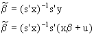
By expanding the multiplication and taking expectations it is obvious that is unbiased.
Now show that has a larger variance.
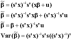
Numerically this is
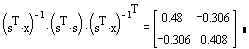
The variance for the OLS estimator is
Although both estimators are unbiased, OLS has the smaller variance in the positive
definite sense. This result is not surprising, given our knowledge of the Gauss-Markov
Theorem.
- A. You can show this several different ways:
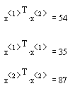
- Compute the inner product of x1 and x2 to show that they are not
orthogonal

Orthogonality is sufficient but not necessary for linear independence.
- Compute the coefficients in the simple regression of x2 on x1 and
show that the residual sum of squares is not zero. LS essentially tries to find the linear
relationship between two variables.

- Compute the determinant of the augmented matrix made from the column vectors x1
and x2.
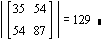
We already knew that the off-diagonals wouldn't be zero, but it is still possible for
the determinant to be zero, which would indicate linear dependence in the columns of x.
2.b. The OLS estimates, using the original data are

2.c. After adding 5 to each obs on y and 10 to each obs on x the OLS estimates are now
Notice that the intercept changed, but neither of the slopes is changed.
2.d. After multiplying each observation on the dependent variable by 10 the OLS
coefficients change to:
2.e. If x1 is multiplied by 10 and the data is otherwise unchanged then the
OLS results change to:

2.f. The effect of adding a constant to both sides of the equation is to change the
intercept. The effect of multiplying the dependent variable by 10 is to rescale all of the
coefficients by a power of 10. Multiplying just one of the independent variables by 10 has
the effect of rescaling only the corresponding coefficient. Notice also, in your
regression output, that R2, t-statistics and the F-statistic are
unaffected by rescaling the data.
3.b. The estimated coefficients are
| Ordinary least squares regression. Dep.
Variable = LNRENT
Observations = 82
Mean of LHS = 0.2020316E+01
StdDev of residuals= 0.3841586E+00
R-squared = 0.9084267E+00
F[ 8, 73] = 0.9052197E+02
Log-likelihood = -0.3313692E+02
Amemiya Pr. Criter.= 0.1027730E+01
Durbin-Watson stat.= 2.2420910 |
Ordinary least squares regression. Weights = ONE Std.Dev
of LHS = .1205161E+01
Sum of squares = 0.1077318E+02
Adjusted R-squared= .89839E+00
Restr.(á=0) Log-l = -0.13115E+03
Akaike Info.Crit. = 0.1637754E+00
Autocorrelation = -0.1210455 |
| ANOVA Source Regression
Residual
Total |
Variation 0.1068723E+03
0.1077318E+02
0.1176455E+03 |
D of Fr 8
73
81 |
Mean Square 0.1335903E+02
0.1475778E+00
0.1452413E+01 |
| Variable |
Coefficients |
Std Error |
t-ratio |
Pr|t|>x |
Mean of X |
Std Dev of x |
| Constant D61
D62
D63
D64
D65
LNMULT
LNMEM
LNACCES |
-0.10446 -0.13980
-0.48911
-0.59385
-0.92482
-1.1632
-.6536E-01
0.57933
-0.14060 |
0.3149 0.1665
0.1738
0.1661
0.1663
0.1661
.284E-01
.353E-01
.293E-01 |
-0.332 -0.840
-2.815
-3.575
-5.561
-7.003
-2.301
16.369
-4.794 |
0.7410 0.4037
0.0062
0.0006
0.0000
0.0000
0.0242
0.0000
0.0000 |
0.14634
0.13415
0.18293
0.21951
0.19512
4.7598
5.7263
1.8266 |
0.35562
0.34291
0.38899
0.41646
0.39873
2.6499
1.5140
2.3422 |
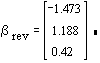
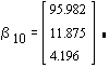
3.b. The quality adjusted price index series is:
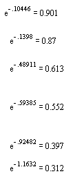
The quality adjusted price index is declining throughout.
3.c. The results for the new model are:
| Ordinary least squares regression. Dep.
Variable = LNRENT
Observations = 82
Mean of LHS = 0.2020316E+01
StdDev of residuals= 0.4907885E+00
R-squared = 0.8423462E+00
F[ 4, 77] = 0.1028530E+03
Log-likelihood = -0.5541066E+02
Amemiya Pr. Criter.= 0.1473431E+01
Durbin-Watson stat.= 1.5506978 |
Ordinary least squares regression. Weights = ONE Std.Dev
of LHS = .1205161E+01
Sum of squares = 0.1854725E+02
Adjusted R-squared= 0.8341564E+00
Restr.(á=0) Log-l = -0.1311522E+03
Akaike Info.Crit. = 0.2555608E+00
Autocorrelation = 0.2246511 |
| ANOVA Source Regression
Residual
Total |
Variation 0.9909821E+02
0.1854725E+02
0.1176455E+03 |
Deg of Freedom 4
77
81 |
Mean Square 0.2477455E+02
0.2408734E+00
0.1452413E+01 |
| Variable |
Coefficients |
Std Error |
t-ratio |
Pr|t|>x |
Mean of X |
Std Dev of x |
| Constant - DUMM1 LNMULT
LNMEM
LNACCES |
-0.57377 -0.60048
-.3732E-01
0.61148
-0.11087 |
0.3856 0.1762
0.353E-01
0.439E-01
0.369E-01 |
-1.488 -3.407
-1.055
13.926
-2.999 |
0.1408 .00105
0.2947
0.0000
0.0036 |
0.8780
4.7598
5.7263
1.8266 |
0.32924
2.6499
1.5140
2.3422 |
The result of using a single dummy for the period 61 to 65 is to increase the magnitude
of each of the slope coefficients, to reduce both the R2 and the adjusted R2
, and the coefficient on LNMULT is no longer different from zero.