Economics 615
Econometrics 1
RV's and Distributions, Hwk 1
| X | 2 | 3 | 4 | 5 | 6 | 7 | 8 | 9 | 10 | 11 | 12 |
| P(X) | 1/36 | 2/36 | 3/36 | 4/36 | 5/36 | 6/36 | 5/36 | 4/36 | 3/36 | 2/36 | 1/36 |
You can derive this easily from enumerating the 36 possible outcomes on the throw of two dice.
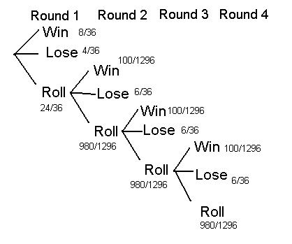
The next step is to diagram the game.
The probability of winning on the first toss of the dice is P(7 or 11)=8/36, the probability of losing is P(2,3,12)=4/36, and the probability of continuing play is then 1-8/36-4/36=24/36.
If you advance to the next round then you must roll a 4,5,6,8,9,10 for a second time in
order to win. There are 6 ways you can win, each with a different probability. The overall
probability of a win in the second round is ![]() . Indeed, each round is identical.
. Indeed, each round is identical.
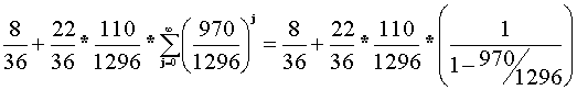
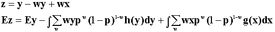
The probability of winning is the sum of winning in the first round plus the probability of winning in the second round + the probability of winning in the third round, and so on. Putting it all together we have

This can be factored as
and is equal to 0.428, approximately. If you bet a dollar to play and receive $1.34 when you win, then the expected payoff is $0.
2. Find the mode.
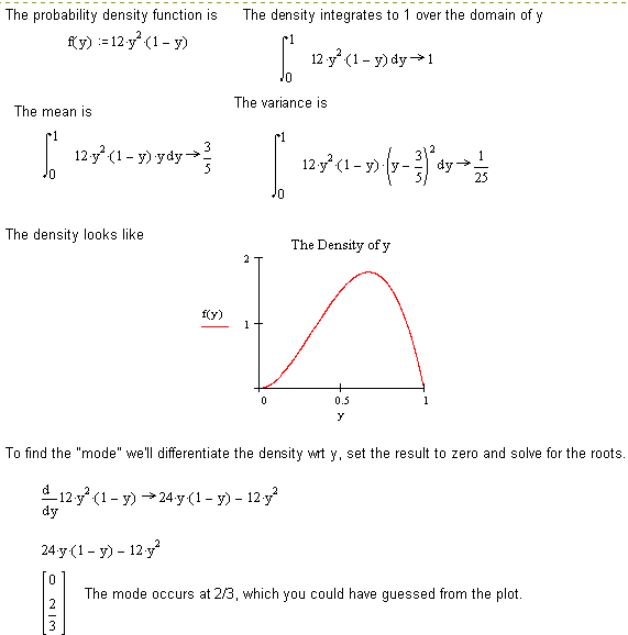
3. This is pretty straightforward.
The last step is obvious.
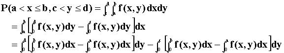
Another way to think of the problem is with the following Venn-like diagram:
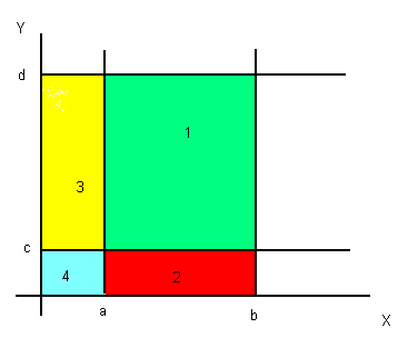
P(a<x<b, c<y<d) = green box 1. Alternatively that probability can be constructed by noting P(x<b and y<d) = Boxes 1+2+3+4, P(x<a and y<c) = Box 4, P(x<b and y<c) = Boxes 2+4, and so on. Now combine the different probabilities to get the desired result.
4. Show that Y1+Y2 and Y1-Y2 are uncorrelated.
Cov(Y1+Y2, Y1-Y2)=E{(Y1+Y2-E Y1-E Y2)( Y1-Y2-E Y1+E Y2)}
=E{((Y1- E Y1)+( Y2- E Y2))(( Y1- E Y1)-( Y2- E Y2))}
If you expand the product in square brackets you will get the difference between two variances, that were to assumed to be equal.
5. The best way to proceed is by first constructing a table:
Y |
||||||||
-1 |
0 |
2 |
3 |
4 |
||||
X |
-1 |
1/6 |
0 |
0 |
1/6 |
0 |
1/3 |
|
0 |
0 |
1/6 |
0 |
0 |
1/6 |
1/3 |
||
1 |
0 |
1/6 |
1/6 |
0 |
0 |
1/3 |
||
1/6 |
2/6 |
1/6 |
1/6 |
1/6 |
1 |
|||
6.a. This is an interesting portfolio construction problem. As you work on this keep the recent bailout of Long Term Capital in mind.
Expand the sums, then the expectations are more obvious.
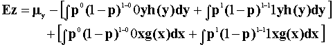
From the square bracket terms we get a weighted average of the mean of y and mean of x.
![]()
![]()
Collect, rearrange, expand the square and take expectations as in part a. to get
![]()
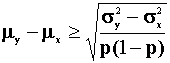
There is a more transparent way to do problem 6. Begin by observing that
W,X, and Y are independent, EW=p, Var(W) = EW2-(EW)2=p(1-p), ![]() .
.
Complete the square, expand the terms, use the independence assumption and recall that EW2 = p.
d. Same as above.