Estimation by Generalized Method of Moments

Overview

Generalized Method of Moments is a class of estimators, or an estimation rule, that includes OLS, GLS and IV estimators as members.  The approach is based on the idea that the population central moments are known functions of unknown parameters of interest.  The population moments can be estimated by the sample central moments.  In turn, the sample moments are then used in place of the population moments in the known system of equations.

Observations about MoM:

1. Except when the random variable being modeled is a member of the exponential family, the method of moment estimators are not efficient.

2. The method of moments is robust to the specification of the data generating process.  The sample mean is an estimator for the population mean, the sample variance is an estimator for the population variance, provided they both exist.

Some Examples of the Method of Moments

x₁, ... ,x_n are independent random variables. Take the functions g₁, g₂, ... , g_n and look at the new random variables

then the y's are also independent. If all the g are the same, then the y are iid.

Now suppose x₁, x₂, ... are iid. Fix k a positive integer. Then are iid and by the weak law of large numbers

which are the k^th moments about the origin.

Define m_k = Ex^k as the k^th moment of x so  and

Suppose you wish to estimate some parameter,.

We know m_k = E(x^k) for k = 1, 2, ... and suppose that is some function of the central moments

and g is continuous.

The sample moment is

Idea: If n, the sample size, is large then should be close to m_k for k = 1, 2, ... , N so should be close to.

Example:

The mean and variance as functions of the first two central moments.

The method of moments estimator foris

, the second sample moment minus the square of the first sample moment.

Example:

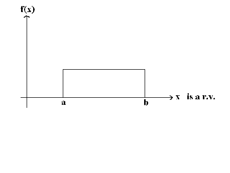
The uniform distribution.

  Consider X, a continuous random variable distributed as the uniform distribution on the interval [a, b]

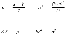
We wish to estimate a and b, the two parameters that characterize the uniform distribution. From experience we know

and

from which we can find the population moments in terms of the parameters of the distribution.  We can then equate the sample moments to the population moments to solve for the unknown parameters of interest.

Suppose = 5 and S² = 2.5

Example:

The inverse Gaussian (Wald) Distribution is used to model elapsed times, e.g, time to failure of a part in a machine.  The shape and location of the density are determined by two parameters, μ and λ. The density is given by

The mean is μ and the variance is  .

A. The efficient maximum likelihood estimators of the two unknown parameters are

 and

B.  The sample mean and sample variance can also be used to estimate the parameters of the distribution as follows:

and

  This follows from the population variance expressed in terms of the central moments.

Example:

The Gamma Distribution has two determinative parameters, P and λ . The density is given by

The Gamma Distribution has as special cases the Chi-square and the Exponential distributions. 

The log likelihood

The mean, m₁, and variance, m₂-m₁², are

from which we can see that

 and

.  One could estimate m₁ and m₂ by the respective sample moments.

Additionally, differentiating the likelihood function with respect to P yields

From Poirier(1995) the moment generating function for the Gamma is

One can differentiate M(t) with respect t and evaluate the result at t=0 to derive an expression for the r^th central moment as

setting r = -1 suggests

We now have four moments and two unknown parameters: m₁, m₂, m_*, m_-1 and P, λ.

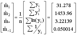
For Greene's income data the results are

Any pair of the sample moments can be used to construct estimates of the two unknowns: four things taken two at a time yields six possible pairs of estimates.  The maximum likelihood estimates are based on m₁ and m_*.

Generalized Method of Moments

Consider the garden variety regression model

                                                                    (1)

We always assume the orthogonality condition

The independent variables and the error term should be independent of one another.  There are k such equations, which are actually moment equations.  The sample analog of this is

This set of coefficients that satisfy these sample moments happen to be the least squares estimates.  We can show the same kind of results for the IV estimator. 

Suppose we know that the orthogonality condition is violated for our model, but we have another set of variables, call them Z, for which the orthogonality condition holds, at least in the limit.

When we have more instruments than unknown coefficients the model is said to over-identified.  The over-identification problem is resolved by solving the following sample moment functions

                                                        (2)

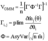
Properties of the GMM estimator

Assumption 1 - The empirical moments converge in probability to their expectation.

Assumption 2 - For any n ≥ k, if θ₁ and θ₂ are two different parameter vectors, then there exist data sets such that m_n(θ₁) ≠ m_n(θ₂) holds for the empirical moments.

A2 ==>  1. The number of moment conditions is at least as large as the number of unknown parameters.
               2. Suppose there are K unknown parameters of the distribution and L moment functions.  The matrix of first derivatives of the moment functions has full row rank.
               3. Any parameter vector that satisfies the population moment condition is unique.

Assumption 3 - If the empirical moments have a finite asymptotic covariance matrix then they converge in distirbution to the normal distribution.

Theorem  Under the three assumptions the method of moments estimator converges in probability to the unknown parameter.  That is, the GMM estimator is consistent.  Also, the GMM estimator is asymptotically distirbuted as a normal random variable.

The theorem allows us to implement, say, an asymptotic t-test or the Wald, Likelihood Ratio and Lagrange Multiplier tests.

The GMM estimator that we have been using is the solution to a criterion function, much like OLS and GLS are the solutions to a criterion function in which the sum of squared errors are minimized.  The GMM criterion function is

Evaluate the three functions at the sample data and multiply by the sample size to get a χ² random variable with L-K degrees of freedom.  L is the number of moment functions and K is the number of unknown parameters.  This test statistic can be used to test the validity of the overidentifying restrictions, and by extension also tests the validity of the underlying model.  In the above example using the Gamma distribution there were two extra moment equations, resulting in six pairs of estimates of the two unknowns.  This specification test can be used to decide whether the six sets of estimates are different from one another.  If they are statistically idfferent form one another then we conclude that the data were not generated by a Gamma.  As another example, in the IV case we often have L>K instruments, resulting in too many orthogonality conditions. If the test statistic described here is large then we conclude that some of the variables used instruments do not qualify as instruments and should have been included as regressors.

The same test statistic

can be evaluated at restricted and unrestricted versions of θ to construct a hypothesis about the parameter vector.

Another interpretation:

Suppose that in (1), above, Ω is not scalar diagonal.  Then it is possible to reinterpret the IV estimator in (2) in an alternative light.  Namely, we choose Z as the triangular square root of Ω^-1, then proceed as with the IV estimator.  In the cases of heteroscedasticity and serial correlation we usually know enough about Ω to estimate it consistently.  Our conclusion is that the method of moments estimator is also heteroscasticity and autocorrelation consistent estimator.

An Example Specific to Economics

Life Cycle Consumption

This example is representative of a whole class of dynamic optimization problems. Suppose that the representative consumer has utility function over consumption each period and tries to maximize

subject to the wealth constraint

where we have the following definitions

E_t = expectation given the information available at time t

δ = rate of subjective tie preference of the consumer

r = fixed real rate of interest

T = length of economic life

C_t = consumption at time t

w_t = earnings at time t

A_t = assets at time t

This model implies and Euler equation of the form

Where U' is the marginal utility of consumption and

The Euler equation can be rewritten as

where the error term ε_t+1 represents the divergence of discounted lagged marginal utility of consumption from its value today.  The error term has mean zero and is serially uncorrelated.  If δ = r, the consumer's rate of time preference is equal to the real rate of interest, then marginal utility would be a constant except for new information arriving between t and t+1.  Hence, the error or innovation to marginal utility is uncorrelated with information arriving on or before period t, this is in the nature of an orthogonality condition.  Let information arriving at time t be represented by Z_t.  Then orthogonality implies

Note that this is in the spirit of a first order condition from an instrumental variables estimator as we saw it earlier in the notes of this section.  Now assume that the utility function is quadratic in consumption, so that marginal utility is linear in consumption.  Accordingly we can write

Following the argument of earlier scholars like Duesenberry or Friedman we might include C_t or Income, y _t , or their lags as instruments.  For the sake of the argument let us construct the instrument matrix as

Zt = [ 1 C_t y_t ]

The test statistic that new instrument is a correctly excluded exogenous variable is

where RSS_R is the sum of squared residuals from the regression of C_t+1 on C_t and a constant, and RSS_A is the residual sum of squares from the regression of the residuals from the restricted regression on income (y_t).

The value of GMM is seen in this example when utility is not quadratic, in which case we could return to the orthogonality condition and estimate.

Robert Hall, "Stochastic Implications of the Life Cycle - Permanent Income Hypothesis: Theory and Evidence" Journal of Political Economy, Vol 86, 1978, Pp 971-987.