Cointegration and Error Correction

Definition: If there exists a stationary linear combination of nonstationary random variables, the variables combined are said to be cointegrated.

The notion of cointegration arose out of the concern about spurious or nonsense regressions in time series.  Specifying a relation in terms of levels of the economic variables, say , often produces empirical results in which the R² is quite high, but the Durbin-Watson statistic is quite low. This happens because economic time series are dominated by smooth, long term trends. That is, the variables behave individually as nonstationary random walks.  In a model which includes two such variables it is possible to choose coefficients which makeappear to be stationary.  But such an empirical result tells us little of the short run relationship between y_t and x_t.   In fact, if the two series are both I(1) then we will often reject the hypothesis of no relationship between them even when none exists.  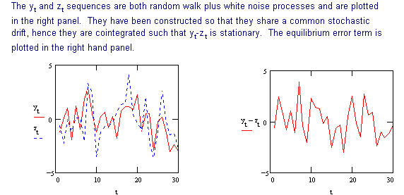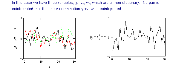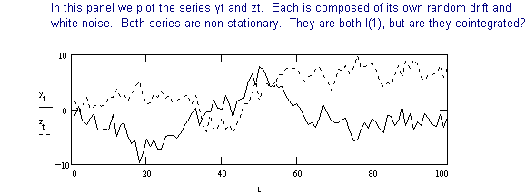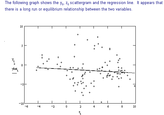For there to be a long run relationship between the variables they must be cointegrated.  The following cases illustrate the discussion:

















To detect cointegration we use the following procedure developed in the previous section.

Procedure:
1. Determine whether y_t and x_t are I(1). This is equivalent to determining whether or not they contain unit roots.
2. Provided they are both I(1), estimate the parameters of the cointegrating relation .
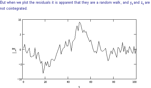
3. Test to see whether the least squares residual appears to be I(0) or not.

Historically, the standard fix-up for overcoming the possibly spurious relationship between two variables has been to first difference each series and redo the regression. This practice has raised the cry that 'valuable long-run information has been lost'.

The problem then is to find a way to work with two possibly nonstationary series in a fashion that allows us to capture both short run and long run effects.  In more technical parlance, cointegration is the link between integrated processes and steady state equilibrium.

For the purpose of illustration we will consider the simple model

in which the error term has no MA part and the cointegrating parameter in the error correction mechanism (ECM, the part in parentheses) is (1, -a).   In the no growth steady state we have and the equilibrium shows a long run proportionality between y_t and x_t when both variables are measured in logarithms.  That is, . Suppose that in the steady state there is a constant rate of growth, say g. That is, .  Then the equilibrium relationship is  .

The procedure for estimating the parameters is to fit the error correction model after having tested for unit roots and cointegration.

To help fix the ideas we consider an analogy.  Sal Minella and her young puppy Spike are seen staggering out of the Charlie Horse Saloon just as we arrive. Sal has had too much to drink. Her movement away from the saloon is seen to be erratic.  Puppies are also prone to wander aimlessly; each new scent provides an impetus to go off in another direction. Dog and owner are not connected by a leash, although Sal knows she owns a dog and Spike will respond to his name.

Sal's meandering down the street can be modeled as a random walk along the real line, .  The real line in this case can be taken to be a narrow path leading away from the bar through an open field.   On coming out of the bar a short time later, our best prediction for Sal's current location is where we last saw her.  Because her movements are a random walk, the longer we have been in the bar ourselves, the more likely it is that Sal has wondered far from where we last saw her.  She is as likely to be on the path as out in the middle of the field.  If the coefficient on x_t-1, her last position, was less than one (in absolute value) then she would tend to return to the path no matter how long we remained in the bar.

Similarly, Spike's wandering can also be modeled as a random walk along the real line, . This equation describes the puppy's random movement from location to location along the path toward home. His movement is also a random walk, so with the passage of time he is as likely to be somewhere on the path as out in the field.

If in her stupor Sal notices that Spike is not at her side she will call his name.   In response he will trot closer to the source of his name.  By the same token, Spike will bark when he realizes that he has wandered off from his mistress and Sal will stagger off in the direction of the bark. Hence we have a long run relationship which recognizes the association between Sal and Spike: . So, although x_t and y_t are both nonstationary, a linear combination of them is stationary. Furthermore, Sal and Spike determine their next 'step' according to the system of equations

The series for the change in, say, Sal's position is determined by the extent to which she and Spike have wandered far apart.  In fact, Sal's next step closes the deviation from long run equilibrium in the previous period by the amount g₂.

Sal and Spike can be generalized to the following definition:

The components of the vector x_t = (x_1t, x_2t, …, x_nt)are cointegrated of order (d,b), denoted by x_t ~ CI(d,b), if

1. All components of x_t are I(d) and
2. There exists a vector b = (b₁, b₂,…,b_n) such that bx_t is I(d-b), where b > 0.

Note b is called the cointegrating vector.   Points to remember:

1. To make b unique we must normalize on one of the coefficients.
2. All variables must be cointegrated of the same order. But, all variables of the same I(d) are not necessarily cointegrated.
3. If x_t is nx1 then there may be as many as n-1 cointegrating vectors. The number of cointegrating vectors is called the cointegrating rank.
   

An interpretation of cointegrated variables is that they share a common stochastic trend. Consider

in which m_it is a random walk and e_it is white noise.  If y_t and z_t are cointegrated then we can write

The term in parentheses must vanish. That is, up to some scalar b₂/b₁ the two variables have the same stochastic trend. The remaining linear combination of the white noise terms is itself white noise.

Given our notions of equilibrium in economics, we must conclude that the time paths of cointegrated variables are determined in part by how far we are from equilibrium. That is, if the variables wander from each other, there must be some way for them to get back together, as in the Spike and Sal example.  This is the notion of error correction.

EXAMPLE

r_st: short term interest rate
r_Lt: long term interest rate

The e_it are white noise. By assumption Dr_it must be stationary, so the LHS variables are I(0). The errors are necessarily I(0). Therefore, the two interest rates must cointegrated of order CI(1,1).

1. We could add lagged Dr_it to the RHS of both equations without changing the interpretation of the model.
2. With the added terms we would have a model similar to a vector autoregression (VAR). However, if we were to estimate an unrestricted VAR then we would introduce a misspecification error.
3. a_s and a_L can be thought of as speed of adjustment parameters.
4. At least one of a_s and a_L must be non-zero.
   

Let us explore the relationship between the error correction model (ECM) and the VAR. Suppose we have the simple model

y_t = a₁₁y_t-1 + a₁₂z_t-1 + e_yt

z_t = a₂₁y_t-1 + a₂₂z_t-1 + e_zt

We can write the model as

Using Cramer's Rule

1. Both variables have the same characteristic equation, in square brackets.  By multiplying  through the equation for y_t, say, by the inverse of [·] you will get an ARMA representation.  In order for the AR part to be stationary the roots of {(1- a₁₁L)(1-a₂₂L)-a₁₂a₂₁L²} must lie outside the unit circle.
2. If the roots of Characteristic equation's (the fraction) polynomial in L (the lag operator) lie inside the unit circle then both z_t and y_t are stationary (see the first point) and cannot be cointegrated.
3. Even if only 1 root of the characteristic equation lies outside the unit circle then both variables are explosive, so cannot be CI(1,1).
4. If both roots are unity then both variables are I(2)and cannot be CI(1,1).
5. If a₁₂ = a₂₁ = 0 and a₁₁ = a₂₂ = 1 then both variables are I(1), but do not have any long run relationship, so cannot be CI.
6. For y_t and z_t to CI(1,1) one root must be 1 and the other must be less than 1.
   

For this particular example we can show

For cointegration either a₁₂ or a₂₁ must be non-zero and the condition that the second root of the polynomial in L be more than 1 in absolute value requires the following condition on the a_ij:

-1 < a₂₂ and a₁₂a₂₁+a₂₂² < 1

Now rewrite the system as



Our prior solution for a₁₁ can be used to write



Make this substitution into the previous line





which can be rewritten as





which is seen to be an ECM.

Implications:

1. If in a VAR the variables are CI(1,1), then an ECM exists.
2. If variables are cointegrated and we wish to estimate a VAR then we must impose restrictions on the VAR coefficients.
3. Suppose y_t and z_t are cointegrated. z_t does not Granger cause y_t if no lagged values of Dz_t-i enter Dy_t and if y_t does not respond to deviations from long run equilibrium.

Testing for cointegration

1. Test the variables for order of integration. They must both (all) be I(d).

2. Estimate the parameters of the long run relationship. For example,

when y_t and z_t are cointegrated OLS is super consistent. That is, the rate of convergence is T² rather than just T in Chebyshev's inequality.

3. Denote the residuals from step 2 as and fit the model

The null and alternate hypotheses are




Interpretation: Rejection of the Null implies the residual is stationary.   If the residual series is stationary then y_t and z_t must be cointegrated.

4. If you reject the null in step 3 then estimate the parameters of the ECM

The terms in parentheses are the error correction terms.  One uses the residuals from step 2 in their place.

EXAMPLE

e_t: the price of foreign exchange in log form



p_t: log of domestic price level

According to the purchasing power parity model (PPP) we should observe that the series

r_t = e_t + p_t^* - p_t

is stationary. In the earlier section on unit roots we observed that this was not the case. As an alternative approach one might argue that the series {e_t + p_t^*} should be cointegrated with {p_t}.  Redefine the foreign price level in dollar terms as f_t = e_t + p_t^*. Then by the PPP model there is a long run relationship

such that u_t is stationary.  Notice that now the cointegrating vector between the three original variables is not (1,1,-1). Now the cointegrating vector between f_t and p_t is



under a strict interpretation of the PPP model.  But such a strict interpretation of the PPP may be too restrictive.

1.  The first step is to see that f_t and p_t are both I(1) for each of the Bundesrepublik Deutschland (BRD), Japan (J) and Canada ( C) relative to the U.S. If they were integrate of different orders then we could reject PPP immediately. For each country the pairs are I(1).  These results are not shown.

2. Fitting the PPP model to the US against BRD, J and C gives us the following result on the slope coefficient, with standard errors in parentheses:

Under the strictest interpretation of the PPP things don't look good for the modelsince the slope coefficients are clearly different from one.

3.  Use the residuals from step 2 to check for unit roots. If f_t and p_t are to be said to be cointegrated then the residual series must be stationary. We fit the models

and

in order to test the hypothesis

H_o: a₁=0, unit root, residual series not stationary, no cointegration

H₁: a₁ not 0, no unit root in residual series, original variables are cointegrated

We must reject the null hypothesis in order to find support for PPP.

We cannot use the usual Dickey Fuller tables since the data are a set of fitted residuals, and at most t-2 of them are independent.

The set of estimates for a₁ are

The numbers in parentheses are 't' statistics.  Only for Japan can we reject the null hypothesis.

Now construct an ECM for the Japan-US model

f_t = .0012 - .1055
(4x10^-4) (4.2x10^-2)

p_t = .00156 + .01114
(3.3x10^-4) (3.17x10^-3)

The numbers in parentheses are standard errors and are the residuals from . For these results, as the foreign price level rises above the domestic price level we will see f_t<0 next period.  If the foreign price level rises above the domestic price level we will see p_t>0 next period.

Note the asymmetry in the data. The speed of adjustment is significant for Japan, but not for the US. At the same time the speed of adjustment is 10x that in the US. This is consistent with the size of the US relative to Japan for the period.

You can dowload another example (a WORD file)for money and income that has both the RATS program and the output.  You can take a look at the data (an EXCEL file) also.