IV. PROPERTIES OF ESTIMATORS
SMALL SAMPLE PROPERTIES
UNBIASEDNESS: An estimator is said to be unbiased if in the long run it takes on the value of the population parameter. That is, if you were to draw a sample, compute the statistic, repeat this many, many times, then the average over all of the sample statistics would equal the population parameter.
Examples:

EFFICIENCY: An estimator is said to be efficient if in the class of unbiased estimators it has minimum variance.
Example: Suppose we have some prior
knowledge that the population from which we are about to sample is normal. The mean of
this population is however unknown to us. Because it is normal we know thatand mediansample
are unbiased

However, consider their variances
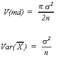
Clearly,is the more efficient since
it has the smaller variance.
SUFFICIENCY: We say that an
estimator is sufficient if it uses all the sample information. The median, because it
considers only rank, is not sufficient. The sample mean considers each member of the
sample as well as its size, so is a sufficient statistic. Or, given the sample mean, the
distribution of no other statistic can contribute more information about the population
mean. We use the factorization theorem to prove sufficiency. If the likelihood function of
a random variable can be factored into a part which has as its arguments only the
statistic and the population parameter and a part which involves only the sample data, the
statistic is sufficient.
LARGE SAMPLE PROPERTIES
Letbe an estimate of
where n denotes sample size.
is a random variable with density
with expectation
and variance
.
As the sample size varies we have a sequence of estimates
a sequence of density functions
a sequence of expectations
and a sequence of variances
Asymptotic theory considers the behavior of these sequences as n becomes large.
We sayis the limiting distribution
of
if for

ASYMPTOTIC UNBIASEDNESS: An estimator is said to be asymptotically unbiased if the following is true
ASYMPTOTIC EFFICIENCY: Define the asymptotic variance as
An asymptotically efficient estimator is an unbiased estimator with smallest asymptotic variance.
CONSISTENCY: A sequence of estimators is said to be consistent if it converges in probability to the true value of the parameter
Example: Define
By the weak law of large numbers we can write
converges to zero as
so the sequenceis a consistent
estimator for
.
IV.B. METHODS OF ESTIMATION
1. METHOD OF MOMENTS
x1, ... ,xn are independent random variables. Take the functions g1, g2,
... , gn and look at the new random
variables
then the y's are also independent. If all the g are the same, then the y are iid.
Now suppose x1, x2, ... are iid. Fix k a positive integer. Thenare iid and by the weak law of large numbers
which are the kth moments about the origin.
Define mk = Exk as the kth
moment of x so
Suppose you wish to estimate some parameter,.
We know mk = E(xk) for k = 1, 2, ... and suppose
and g is continuous.
The sample moment is
Idea: If n is large thenshould be close to mk for k = 1, 2, ... , N so
should be close to
.
Example:

The method of moments estimator foris
Example:
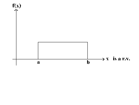
X is a continuous r.v. distributed uniformly on the interval [a, b]. We wish to estimate a and b. From experience we know
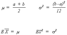
Suppose = 5 and S2 = 2.5
LEAST SQUARES
We have an unknown mean . Our
estimator will be
. Take each xi, subtract its predicted value, i.e. its mean,
square the difference and add up the squared differences
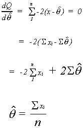
This is nothing more than , which we
know to be the least squares estimator of
for any distribution.
MAXIMUM LIKELIHOOD ESTIMATORS
Suppose we have the random vaiable xi with the following density function
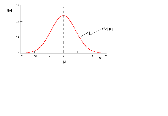
The position of the density function depends on. The likelihood function is found by holding the statistic constant and
letting the parameter vary.
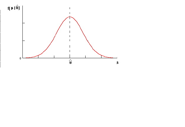
While the overall picture does not look different, there are some fundamental alterations in the way it is labeled. See figure 2.
Notice that in the revised figure the domain is now m
and the range is conditional on the sample statistic . We choose that value for the parameter which makes it most likely to have
observed the sample data.
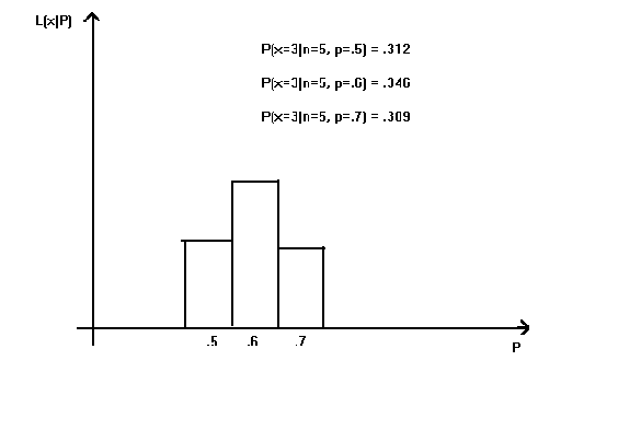
Example: We have a binomial and we wish to estimate P. The sample size is n = 5. Choices for the probability of success are P = .5, .6, .7. We do the experiment and find x = 3. Let us vary P and compute the probability of observing our particular sample. Given the results shown in figure 3, would you ever choose either .5 or .6 as the best guess for the true proportion P?
Example: You are a medieval serf and wish to marry the Queen's son. You must plunge your hand into an urn of balls numbered consecutively 1, 2, 3, ... to some unknown maximum. If you guess the number of balls in the urn then you are permitted to marry the prince. q is the number of balls in the urn. You have drawn out a ball with the number 27 on it. What is your guess for the total number of balls?
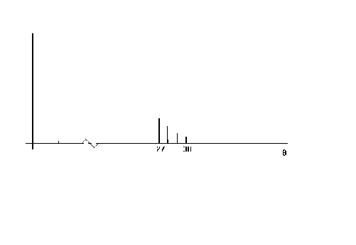
Would you ever guess a number greater than 27? Were you to do so then the probability of drawing a 27 would decline.
Example: We don't know the
particular that applies to a steel rail
production process. Wishing to estimate
, we
observe 5 flaws in one mile of rail, x = 5 so,
One approach to estimating the rate parameter would be to construct the probability
distribution for different possible values. This is done in the figure below.
Figure 5
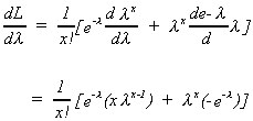
A more efficient way to estimate the rate parameter is as follows
set the derivative to zero and solve for.

IV. C. CONFIDENCE INTERVALS
It should be noted that the probability of a point estimate being correct is zero! Consequently, we construct more practical interval estimates.
Consider the first sample mean problems we dealt with
where. This can be rewritten as
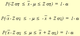
This is called aconfidence interval.
Note: 1. is a fixed number
2. is a random variable
As long as we do not plug in numbers we
can leave this in the form of a probability statement.
Example: Suppose. We observe
for n = 81
is a 95% confidence interval.
INTERPRETATION: Of all confidence
intervals calculated in a similar fashion {95%, n=81} we would expect that 95% of them
would cover.
does not change, only the position of the interval. Think of a big
barrel containing 1000 different confidence intervals, different because they each use a
different value of the random variable
. The
probability of us reaching in and grabbing a "correct" interval is 95%. But, as
soon as we break open the capsule and read the numbers the mean is either there or it
isn't.
In the above construction it was assumed that we knew. Suppose we don't know
or
but still wish to construct
an interval estimate.
Example: We know. From a sample of size 25 we observe
and
. To construct a 95% confidence interval for
is a 95% confidence interval.
There are three other cases that we could encounter:
a. Distribution of x unknown,known
and sample size large - Rely on CLT to use
b. Distribution of x unknown,unknown
but n large - technically should use t but z is a fair approximation.
c. Distribution of x unknown,unknown,
n small - STOP.
To help keep the three cases straight we have another flow diagram.
IV.C.2. CONFIDENCE INTERVALS FOR
Recall
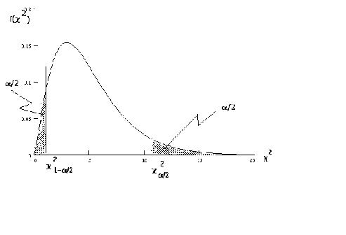
As in our use of Z and t in constructing a confidence interval forwe must choose two
values. This is done as per the below diagram
From the above recollection
Substitute this into the above probability statement
Rearranging
Note that s2 is the random
variable. When numbers are plugged in it is no longer appropriate to express the interval
as a probability statement.