As before we posit Y = Xb + U with r(X) = k < n and X is uncorrelated with the error term. But now we generalize the assumptions about the error term a little bit.

Generalized Least Squares
In this chapter we generalize the results of the previous chapter as the basis for
introducing the pathological diseases of regression analysis. First, we abandon the
assumption of a scalar diagonal variance of the error term, but find that with certain
modifications a least squares estimator is still BLUE. Subsequently we consider
heteroscedasticity and autocorrelation. In these subsequent sections we examine the
consequence of the violation of the classical assumption, the detection of the problem,
and a proposed remedy for the problem.
The Aitken Estimator
As before we posit Y = Xb + U with r(X)
= k < n and X is uncorrelated with the error term. But now we generalize the
assumptions about the error term a little bit.

We assume that the error term still has a mean of zero. Although the error variance is
not scalar diagonal, we do know its structure up to a scalar constant. It remains
symmetric and positive definite.
Under the present assumptions
is the BLUE for our posited model. We can prove this as follows
So at the very least this estimator is unbiased and linear in Y.
Turning to the variance
Using the construction of the Gauss-Markov Theorem we could easily show that no other
linear unbiased estimator has a smaller variance.
How about an estimator of the unknown s2? Well
is a natural since, by substitution,
shows our choice to be unbiased.
At the outset it was assumed that the error covariance matrix was known up to the scalar s2. This is a
rather strong assumption. In its absence we have another n(n+1)/2 unknowns to estimate.
This would in all likelihood be well beyond the capabilities of our data. The result is
that we often make specific assumptions about the structure of the error covariance
matrix. In any event, once we have made an assumption about the structure of W it may be possible to estimate it consistently. When we have a
consistent estimator to use in place of W in the GLS estimator
then we can show that the slope coefficient estimator is consistent.
The following curiosities are of more than passing interest.
(i) Because of the way regression packages are programmed they automatically and by
default give you the following
Since this is the least squares estimator it remains unbiased, although the computer has
given it to you inadvertantly. However, when the error covariance matrix is not scalar
diagonal, the OLS estimator is no longer efficient.
The variance of the OLS estimator must be greater than that of the GLS estimator by the
Gauss-Markov Theorem.
(ii) If plim(X'X)-1 = 0 then OLS is consistent.
(iii) We can also show that OLS is asymptotically normal.
Heteroscedasticity
While reading you should keep in mind several questions: What is
heteroscedasticity? What are the consequences for OLS? How does one detect it? Ow does one
correct for it? As a pathological disease, heteroscedasticity impacts the disturbance
term. Typically we assume EUi2
= s2
for all i in the sample. That is, the error term is homoscedastic; all errors have the
same variance.
Consider the case where we observe a number of firms at the
same point in time. It is reasonable to expect that the error corresponding to larger
firms will have a bigger variance than that for the smaller firms. Or consider attempts to
estimate income elasticites on the basis of a cross section. For any commodity, we would
expect more variability in consumption from the higher income group.
We shall begin with a rather general discussion. We posit
Y = Xb + U
and
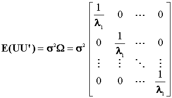
we will assume s2
is not known and W is a known, symmetric and positive definite
matrix. Now define
Then P-1'P-1 = W-1.
According to our previous work with the Aitken estimator we find
to be BLUE and its variance is given by
If we already know W then we should transform the model by P-1. That is P-1Y
= P-1Xb + P-1U
So that when we construct the least squares estimator from the transformed data we get
It is only in special circumstances that we know the specific form of W.
When the error covariance is not scalar diagonal and we apply OLS anyway the estimator is
not efficient. That is, there is a linear unbiased estimator with smaller variance. The
inadvertant use of OLS, and its attendant large standard errors (small t statistics) will
lead us to conclude that a variable is not significantly different from zero.
An example of correcting for heteroscedasticity follows.
EXAMPLE
Consider a standardized exam and parent's income. We propose
qij = a + bxij + uij (1)
for i = 1, 2, ... , nj and j = 1, 2, ... , m
where qij is the test score of a particular
student from the jth school and xij is his
parent's income. There are m schools with nj
students in each. The error term is thought to be homoscedastic.
As a result of privacy laws we do not observe individual scores and income. Rather, we
observe the average score for the school.
is the average score of the students in the school and
is the average income of parents in school j.
Note that the schools are of different sizes. Therefore it will be necessary to weight the
observations.
The model we are really using is
Qj = a + bXj + Uj
(2)
j = 1, 2, ..., m
The error term in the more crass model is characterized by
Because the denominator is different for each school, the variance of each Uj
will differ. While OLS will still be unbiased, it will not be efficient. What can we do to
make our estimates of a and b as
good as possible? Begin by finding the error variance for the crass model.
Using these results to put together the whole error covariance matrix
We must correct for the different variances on the diagonal. If we properly weight the
observations we can get a scalar diagonal covariance matrix. Define
Now transform the data as follows
By rescaling the data in this fashion we arrive at the following conclusion regarding
the error term
Therefore is BLUE.
Testing for Heteroscedasticity
Goldfeld Quandt Test
It behooves us to have a method for determining when we have the disease
of heteroscedasticity. Goldfeld and Quandt suggest the following test procedure.
1. Choose a column of X according to which the error variance might be ordered.
2. Arrange the observations in the model in accordance with the size of Xj.
3. Omit an arbitrary number, say c, of central observations from the ordered set. Make
sure (n-c)/2 > k.
4. Fit separate regressions to the first (n-c)/2 observations and to the next (n-c)/2
observations.
5. Define for the residuals from the case where Xj are
small and
for the residuals from the case where Xj are
large.
6. Let F = RSS2/RSS1. This has an F distribution with (n-c)/2-k
degrees of freedomn on numerator and denominator.
The hypothesis we are testing is
Ho: F = 1
H1: F > 1
If we observe a large F then we reject the null.
Replicated Data
This particular problem is most often seen in the natural sciences. A classic example to
be found in economics is Nerlove. The idea is that we have several observations
(i=1,2,...,ni) for each size
class of firms and there are m size classes. The model is yij = a + bxij + uij i=1,2,...,m; j=1,2,...,ni with the assumptions
If we stack the data then the model is written as 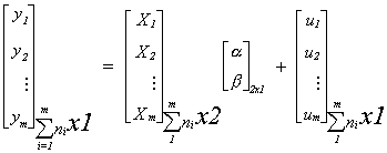
The subscripts on the braces show the dimensions of the various matrices. Note the
implied restriction that the intercept and slope are equal across groups. Look for this
question to come up in the sections on seemingly unrelated regression and random effects
models. In this revised form the error covariance for the entire disturbance vector is
written as
The hypothesis to be tested is 
The test procedure is as follows
1. Pool the data and estimate the slope parameters by OLS.
2. From the entire residual vector, e, estimate the pooled least squares residual
variance,

Note that you are using the maximum likelihood estimate of the error variance under the
null hypothesis.
3. For each group or class in the sample construct an estimate of the error variance from
4. Construct the test statistic
5. For large observed test statistics we reject the null hypothesis.
Glejser Explorations
Glejser offers an approach to the heteroscedasticity problem based on running some
supplementary regressions.
Procedure:
1. Estmate the parameters of Y = Xb + U. Obtain the least
squares residuals, ei.
2. Estimate the parameters of
3. Construct a test of the hypothesis
Breusch-Pagan
Breusch and Pagan offer an extension to the work of Glejser. Essentially they provide a
test to help the researcher decide whether or not s/he has solved the heteroscedasticity
problem.
Once again the model is Y = Xb + U, but with
the a are p unknown coefficients and the zi are a set of variables thought to affect heteroscedasticity. The null hypothesis is that apart from the intercept the ai are all zero, Ho: a2=a3= ... =ap=0.
Procedure:
1. Fit Y = Xb + U and obtain the vector of OLS residuals, e.
2. Compute the maximum likelihood estimator for s2 and a variable that we will
use as dependent variable in a supplementary regression.
3. Choose the variables zi then estimate the coefficients of
and obtain the residuals.
4. Compute the explained sum of squares from the regression in step 3.
5. From the explained sum of squares construct the test statistic
The null hypothesis of homoscedasticity is rejected for large values of Q.
White's General Test
White's test has become ubiquitous. It is now programmed into most regression packages,
both the test and the correction. The correction computes the proper estimate of the
variance when one applies OLS in the presence of heteroscedasticity. This correct variance
is then used in tests of hypothesis about the slope parameters.
Recall that the correct covariance matrix for the least squares estimator is . This can be consistently estimated by
where xi is the transpose of the ith row of X, so it has
dimension kx1 and xi' has dimension 1xk. The default estimator used by most
regression packages is . Which is, of course, not
consistent when the errors are heteroscedastic.
To conduct the test for homoscedasticity use the following procedure
1. Apply OLS to the original model and construct ei2 from the
residuals.
2. Estimate the parameters of the following regression model:
The set of right hand side variables are formed by finding the set of all unique variables
formed when the original independent variables are multiplied by themselves and one
another.
The test statistic is formed from the simple coefficient of determination in step 2. That
is,.
Spearman's rank Test
A nonparametric test is offered by Spearman. Suppose you have the model yi =
xib+ui. First estimate the model
parameters and save the residuals. For the sake of the example, we believe the variance of
ui to be related to the size of the observation on x. If they are directly
related then the rank of the ith obervation on x, say dix,
should correspond to the observed rank diu. Hence, one would expect
the differences in the ranks for x and u to be zero on average. Let the squared difference
for the ith observation be
and construct the correlation coefficient

If the rank orderings are identical for x and u, then rs will be one.
As with any correlation coefficient, we can do a t-test
As a pathological disease, autocorrelation also impacts the disturbances. Contrary to
the original assumption about our regression model, we now allow the error in one period
to affect the error in a subsequent period. Consider the model Yt = Xtb + Ut where is the serially correlated error. We assume the following about et and r
The et
term is known as white noise; it has constant mean and variance for all periods and is not
serially correlated. Since r is nonzero it introduces some
persistence into the system when there are shocks from the white noise term.
We can expand our expression for Ut
By continuous substitution
The current disturbance is a declining average of the entire history of the white noise
term. In order to say anything about the use of OLS in the presence of autocorrelation we
need to find the mean and variance of the disturbance.
MEAN
Since the RHS is a linear combination of random variables all with mean zero, the
disturbance has a mean of zero.
VARIANCE
Upon taking expectations the terms under the double sum are all cross products and drop
out. That is, their time subscripts do not match and we have assumed that there is no
serial correlation in the white noise term. Thus, using a bit of our human capital about
infinite series,
We also need to be able to say something about the covariance between the current
disturbance and past disturbances in order to build up the entire error covariance matrix
for the sample.
Note the following
Applying the same tricks of the trade that we used for the expectation of Ut2
we find
We could apply the same tricks ad nauseum for all the possible offsets in time
subscript and arrive at the following
Putting everything together in an error covariance matrix gives us
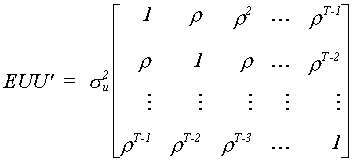
Let us now consider the effects of autocorrelation on our conventional OLS estimator.
Consequences of Autocorrelation for OLS
BIAS
Therefore autocorrelation leaves OLS unbiased.
VARIANCE OF OLS
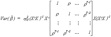
In order to shed more light on this we will consider the very simple model yt
= bxt + ut with
and make x a column vector
Using our earlier results on the form of the covariance matrix for the OLS estimator
If you persist and do the multiplication then once the smoke clears you will arrive at
Recall that your regression package always reports for the variance of the least squares estimator. Which is larger, the
variance reported by the machine or the correct variance of the OLS estimator?
In the usual autocorrelation case 0 < r < 1. If you look
closely at each term of the variance for our example you will see that each fraction looks
like the estimate of a regression coefficient. That is
Usually 0 < y. In fact, it is often the case with
economic time series that we find y is approximately one. We
conclude then that the machine reported estimate of the variance understates the true
variance. The implication is that if we fail to detect and correct for autocorrelation and
rely on the machine reported coefficient covariance then
o when calculating confidence intervals they will appear more precise than they really are
o we will reject more Ho than we should.
In spite of any problems with the dunderheaded computer, OLS remains unbiased. If , where xt' and xs' (of dimension
1xk) are rows of X, converges to a matrix of finite elements then OLS is consistent. The
import of this requirement is that you had better not include a time trend in your time
series model! The OLS estimator also remains asymptotically normal under most
circumstances. The caveat emptor, as in the heteroscedasticity case, is that OLS is not
efficient.
Testing for Serial Correlation
Durbin-Watson Test for Autocorrelation
D-W suggest
D-W have shown the following
1. When r = 0 then = 2.0
2. When r > 0 then < 2.0
i.e. positive autocorrelation
3. When r < 0 then > 2.0
i.e. negative autocorrelation
4. 0 < < 4
Unfortunately, the distribution of depends on the matrix of independent variables, so is
different for every data set. We can characterize two polar cases.
A. X evolves smoothly. That is, the independent variables are dominated by trend and long
cycle components. If you regress a given variable on its own one period lag the slope
coefficient would be positive.
B. X evolves frenetically. That is, the independent variables are dominated by short
cycles and random components. If you regress a given variable on its own one period lag
the slope coefficient would be negative.
For the case when r > 0 the situation is pictured below.
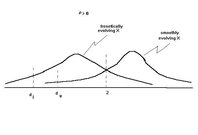
As a result of the two polar cases there will be two critical values for the test
statistic, dl and du. Since we never know whether our data evolves
smoothly or frenetically we have a "no man's zone" in the reject region. If the
observed value of the Durbin Watson statistic is less than dl, then we can
state unequivocally that the null should be
rejected. If the observed Durbin-Watson is above du then we can state
unequivocally that the null should not be rejected. But if is between dl and du
then we must punt.
Apart from the "no man's zone", there are a few other problems with the Durbin
Watson statistic. First, the null is against a specific alternative. The consequence is
that if the error process is something other than AR(1) then the DW is easily fooled.
Secondly, the DW critical tables are set up assuming that the researcher has included an
intercept in his model. Thirdly, one cannot use the DW to test for an AR(1) error process
if the model has a lagged dependent variable on the right hand side.
When there is a Lagged Dependent Variable
Suppose we have
with
Then the appropriate test statistic is 
and
.
Wallis' Test for Fourth Order Correlation
Suppose we have a quarterly model, then the error specification is likely to be and we wish to test the null
. The test
statistic will be
The tabulated critical vaoues are in Wallis, Econometrica, Vol. 40, 1972 or Giles and
King, Journal of Econometrics, Vol. 8, 1978.
Breusch-Godfrey Tests Against More General Alternatives
The null hypothesis is that the model looks like
The alternatives against which we can test are
where, under the alternatives, .
Procedure
1. Construct the OLS residuals .
2. Construct the MLE for su2
and
3. Construct the test statistic
reject the null for large values of the test statistic.
NOTE: The part in square brackets is a pxp matrix. The elements on the main diagonal are
residual sums of squares from the regression of the columns of Ep on the column
space of X. With this in mind, the procedure outlined here is equivalent to checking TR2
for
against an appropriate critical value in the c2
table.
What to Do About Autocorrelation {AR(1)}
Although we will do the case in which the error term is AR(1), it is true that AR(1)
and MA(1) are locally equivalent. The basic model is Yt = Xtb + Ut with Ut = Ut-1+t
Begin with
Substitute the error structure into (1) and multiply (2) by r
and subtract the result from (1) to get
Since Eet = 0 and Eee' = s2I we have an equation with no autocorrelation. If we
knew r we could easily estimate the parameters of this well
behaved model.
Define DYt = Yt - Yt-1, the
first difference, and DrYt = Yt
- rYt-1, the partial difference.
DURBIN'S METHOD
The well behaved model is Yt - rYt-1 =
(Xt - rXt-1)b
+ et,
rewrite this as Yt = rYt-1 + Xtb - rXt-1b
+ et
Estimating the parameters of this model gives an estimate of r.
Use the estimate of r to construct the partial differences and
reestimate the model parameters. The Durbin process is best for small samples.
TWO STEP COCHRAN-ORCUTT METHOD
1. Estimate the model parameters with OLS.
2. Calculate an estimate of r from
3. Partial difference all of the data using the estimate of r.
4. Estimate the model parameters of
using OLS.