6. Simultaneous Equations
6.1 The Problem

6.1.1 Graphical Views of the Identification Problem

A Three Dimensional View of Supply and Demand
A Two Dimensional View of How the Data are Generated
In both graphical views you should have noticed that fitting a line by OLS to the observed data will incorrectly estimate the unknown slope coefficient. If you didn't catch this, go back and look again.

6.1.2 A Specific Example

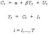
Consider the simple macroeconomic model
(6.1)
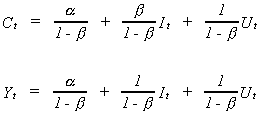
C is consumption, Y is real GDP and I is investment and is assumed to be non-stochastic. Substituting and solving for the two behavioral variables
(6.2)
In our model (6.1) is known as the structural system and (6.2) is known as the reduced form.
The first problem that we encounter in systems models is best addressed by rewriting the reduced form and doing a bit of tedious algebra.
(6.3)
Applying OLS to these equations we can estimate the set of ps consistently since the RHS variable is independent of the error term. Referring back to (6.2) we see that we can construct an estimate of b from two different equations. For this example the numerical results will be identical. Can you prove it?

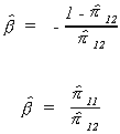
In this example in which the two numerical results are the same we are lucky, the first equation is said to be identified.
The second problem that we encounter in systems models has to do with properties of estimators. It is illustrated by continuing the example. Suppose that we apply OLS to (6.1) to obtain an estimate for b

Both Yt and Ct are random variables so it is hard to evaluate . We can, however, evaluate the probability limit.

Consider first the denominator

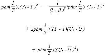
which was derived by substituting from (6.2). So



Turning now to the numerator


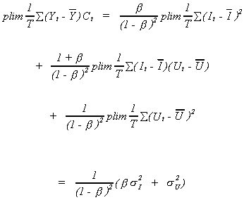
Putting the pieces back together

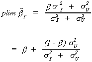
In the context of the model we are considering, we know that the MPC, b, is between zero and 1. We can see from the above result that even in large samples we over-estimate b.

A simple graphical representation shows the effect of the consistency problem on the magnitude of over-estimation.

To summarize the results of this section, we have seen that we can always estimate the parameters of the reduced form consistently. This is not necessarily the case for the structural form. If it is possible to consistently estimate the parameters of the reduced form, under what circumstances can we construct point estimates of the structural parameters form the reduced form results? When is there enough information in the reduced form to just identify the structural parameters? If the application of least squares to the reduced form provides too much information, are there alternative estimation techniques which enable us to use the excess?

In what follows we explore the two problems of systems models in greater detail. In the next section we explore the identification problem. After that we take up different methods of estimation. In the final section we consider some special testing procedures for systems models.

1. Identification
   

The classic paper in this area is E.J. Working, "What Do Statistical Demand Curves Show?" Quarterly Journal Of Economics, Vol. 41, No. 1, February 1927. The most definitive treatment is Franklin Fisher, The Identification Problem in Econometrics, Robert E. Krieger Publishing Co., Huntington, N.Y., 1976.

In this section we begin by introducing some notation. Then the problem of identification is introduced by exploring three simple cases. From there we go to a more general treatment with retrospective looks at the three special cases.
Suppose we have the structural model

The first subscript identifies the variable, the second subscript identifies the equation. Thus, we have the same number of endogenous variables as we have equations, m. There are k exogenous variables. Converting to matrix form we can write

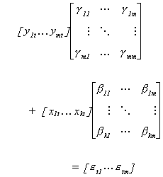
Be sure to note that the columns of the coefficient matrices correspond to the structural equations. Also, an observation on all the variables is arranged as a row. In order to avoid having to write so much, we write the structural model as

We proceed as follows to get the reduced form

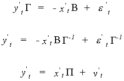
Can you state the order of all the matrices in this representation? In terms of all the observations the structural model can be written

The subscripts indicate the dimensions of the matrices.
We turn now to a specification of the error variance. For the structural model we have

S is an mxm matrix of contemporaneous covariances between the equation error terms.
For the reduced form we have






Identification by Exclusion Restrictions

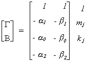
EXAMPLE 1 An Underidentified System
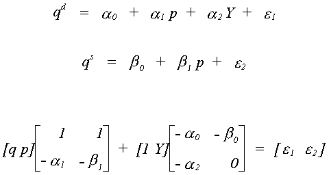
We have a demand equation and a supply equation, respectively:

in which the exogenous variables are denoted by Z, and the endogenous variables are P and q. Writing things in matrix form

The reduced form is found as follows

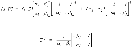
After doing all the algebra we come up with

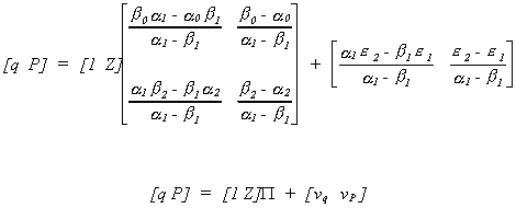
Note:
1. We have four equations in six unknowns from the reduced form equations.
2. Alternatively

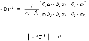
The rank of the matrix of the reduced form coefficients is not 2, it is only 1.
3. Also, in each equation of the structural model we have 2 included endogenous variables and no excluded exogenous variables.
The issue of rank and counts of included endogenous and excluded exogenous variables will prove crucial in our discussion of the identification problem.

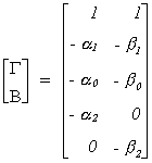
EXAMPLE 2 An Exactly Identified System

Writing things in matrix form

The reduced form is as follows

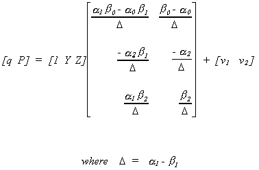
Note:
1. Now we have 6 equations and 6 unknowns from the reduced form.
2. The rank of is 2 and the number of endogenous variables is 2.
3. In each structural equation we have an excluded exogenous and 2 included endogenous variables.

EXAMPLE 3 An Overidentified Macroeconomic Model

The model has three equations. Two of them are behavioral: consumption, c, and investment, i. The third is the national income,y, identity that expenditures must equal income in equilibrium. The exogenous variables include the interest rate, r, government spending, g, lagged consumption, c_-1, and lagged income, y_-1. The structural model is

Since the last equation is an identity, e₃ is a degenerate random variable. That is, its variance is zero.
The reduced form, which you could derive with a pencil and paper or using a program like Mathematica or MathCAD, is as follows

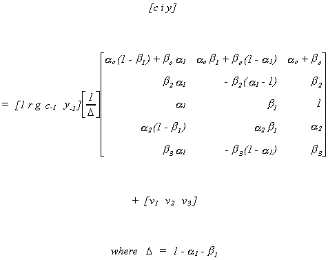
Note:
1. There are 15 equations in 7 unknowns in the reduced form.
2. The rank of P is three and there are three endogenous variables.
3. There are two included endogenous variables in each equation of interest. The first equation has 3 excluded exogenous, the second has equation has 2 excluded exogenous, and the third equation has 4 excluded exogenous variables.


THEOREM: The Order Condition
k^*_j ³ m_j
The number of excluded exogenous variables must be greater than the number of endogenous variables found on the right hand side of equation j.
This theorem is a straightforward matter of counting. It is a necessary but not sufficient condition for an equation to be identified.
Before we can introduce The Rank Condition we need some new notation for the reduced form equations. Everyone knows you can't tell the players without a scorecard. The following table provides some vital statistics for the elements of the reduced form shown below the table.

Player	Description	Dimension
yj	dependent variable in the jth structural equation	1 x 1
Yj'	endogenous variables on the "RHS" of the jth structural equation	1 x mj
Y*j'	endogenous variables NOT appearing in the jth structural equation	1 x m*j
xj'	included exogenous variables of the jth structural equation	1 x kj
Xj*	excluded exogenous variables of the jth structural equation	1 x kj*
pj	reduced form coefficients on the exogenous variables included in the jth structural equation	kj x 1
pj*	reduced form coefficients on the exogenous variables excluded from the jth structural equation	kj* x 1
	coefficients of exogenous variables, # of rows corresponds to the number of included exogenous variables in the jth equation, # of columns corresponds to the number of included endogenous variables in the jth equat ion	kj x mj
	coefficients of exogenous variables, # of rows corresponds to the excluded exogenous variables of the jth equation, # of columns corresponds to included endogenous variables	kj* x mj
	coefficients of exogenous variables, # of rows correspond to included exogenous variables, columns correspond to excluded endogenous variables	kj x mj*
	coefficients of exogenous variables, rows correspond to excluded exogenous and columns correspond to excluded endogenous variables	kj* x mj*
vj	reduced form error corresponding to the LHS variable of the jth structural equation	1 x 1
Vj'	reduced form error vector corresponding to the RHS endogenous variables of the jth structural equation	1 x mj
Vj*	reduced form error vector corresponding to the endogenous variables excluded from the jth structural equation	1 x mj*

The left hand side of the system of reduced form equations has been partitioned according to whether and where an endogenous variable is included in the structural form. The right hand side has then been partitioned conformably.

Recall that so we can write the matrix of endogenous structural coefficients as . The j^th column of B corresponds to the j^th structural equation. To get these we need just the j^th column of G.

Now G_j is the set of coefficients for the endogenous variables of the j^th structural equation, or

Combining this with our representation of the partitioned reduced form we get

Carrying out the multiplication allows us to write this as two equations The second equation gives us a system of k_j^* non-homogeneous equations in m_j unknowns. The order condition follows from this obviously. From linear algebra we know that there is a unique solution, to the system of non-homogeneous equations if and only if Rank() = m_j.

THEOREM: The Rank Condition

The jth equation is identified IFF Rank() = m_j. That is, the rank of the k_j^* x m_j matrix of reduced form coefficients corresponding to include endogenous - excluded exogenous variables must be m_j.

Example 4 (Example 1 again)

We can interpret the above using Greene's terminology. The coefficients of the j^th equation have been moved to the first column. The coefficients of the remaining equations are in the last m-1 columns. The rows have been rearranged according to the dependent variable, the included endogenous variables, excluded endogenous variables, included exogenous variables, and excluded exogenous variables. The first row of the remaining columns corresponds to Green's A₁, the next row corresponds to A₂ (included endogenous variables), there is no A₃ (excluded endogenous), the final k_j=2 rows correspond to A₄ (included exogenous), there is no A₅ (excluded exogenous).
Since m_j^* = 0 and k_j^* = 0 neither equation is identified.

Example 5 (Example 2 again)

The coefficients of the j^th equation have been moved to the first column. The coefficients of the remaining equations are in the last m-1 columns. The rows have been rearranged according to the dependent variable, the included endogenous variables, excluded endogenous variables, included exogenous variables, and excluded exogenous variables. The first row of the remaining columns corresponds to Green's A₁, the next row corresponds to A₂ (included endogenous variables), there is no A₃ (excluded endogenous), the next 2 rows correspond to A₄ (included exogenous), the last row is A₅ (excluded exogenous).
Note m_j^* = 0 and k_j^* = 1. A₅ has rank 1, equal to the number of included endogenous variables so the equation is identified.

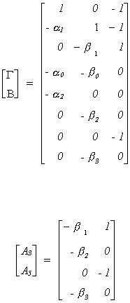
Example 6 (Example 3 again)

The matrix of coefficients has been rearranged using Greene's scheme. First, the coefficients of the equation of interest are moved to the first column. Then the rows are rearranged. The first row is the row of the dependent variable, A₁. The second row carries the included coefficient of the included endogenous variable, A₂. The third row is the excluded endogenous variable, A₃. The fourth and fifth rows are for the included exogenous variables, A₄. The final three rows correspond to the excluded exogenous variables, A₅.
The augmented matrix (A₃, A₅) has rank 2 and there is one included endogenous variable. The first equation is over identified.

Identification by Covariance Restrictions

We return to the underidentified supply and demand model.

We want to see if it is possible for there to be a false structure. That is, can we find a set of restrictions that provides us with two equivalent structures. Or, BF = B^*, where B^* must have the same pattern of zero and nonzero terms as B.

So we conclude that f₁₂ = 0.

The covariance for the false structure is

Suppose we know that s₁₂ = s₂₁ = 0. Then

Since f₁₂ = 0 it must be that either f₂₁ = 0 or f₂₂ = 0. If the latter is true then there would be no second equation so we conclude that f₂₁ = 0 and the only admissible value for f₁₁ and f₂₂ is one.
Recall that the reduced form for the model is

For the supply equation

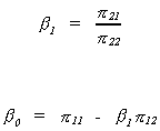
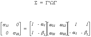
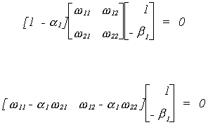
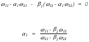
We know the relationship between structural and reduced form covariances to be

Since we are interested in only off diagonals we need not do all of the multiplication

And then

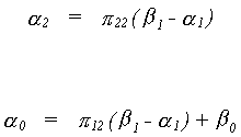
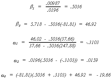
Using the data in Greene we can complete the example as follows

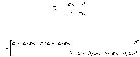
For the structural error covariance matrix


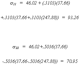
Using the data in Greene we can calculate the equation variances as shown below.