DATA PROBLEMS: Multicollinearity

Multicollinearity is one of the most widely taught of all the pathological diseases of econometrics. It is also one of the more frequently misunderstood of the pathological diseases. I believe this to be the case because on the surface it is conceptually a very simple idea. When we look a bit further, symptoms that we ascribe to multicollinearity may be the result of something else.  Similarly, we may be misled by the usual diagnostics.  When you are done reading this section of the notes, go to "Explorations in Multicollinearity."

We begin with the usual model y = xb + u.  y and u are nx1, x is nxk, and b is kx1. The error term is well behaved. There is no correlation between the independent variables and the error term.  If where u_i is a "stochastic" term, with finite mean and variance, and not all the l_i are zero then we have a problem of multicollinearity. That is, there is some linear dependence, albeit not exact, between the columns of the design matrix. This defintion is already problematic. The classical assumption of regression analysis is that the columns of the design matrix are linearly independent; they span a vector space of dimension k; the matrix x'x has k non-zero roots. The model and the experiment are designed so that the independent variables have separate and independent effects on the dependent variable. With economic data the experimant usually cannot be reproduced or redesigned, in spite of the fact that a common assumption that x is fixed in repeated samples.. The data is not always well behaved.

What if the linear dependence, while not exact, is close? What if one of the roots is very small and another very large? What if one of the explanatory variables doesn't have much variation in it? In the sense of linear algebra the matrix x will still span a vector space of dimension k. That is, we can estimate the parameter vector b, but not very precisely.
Our problem is a sample phenomenon. The sample may not be rich enough to allow for all the effects we believe to exist.

Classic Multicollinearity and Imprecision of OLS

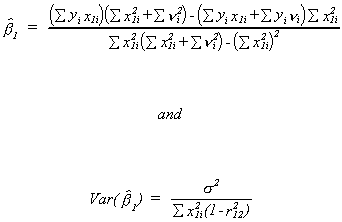
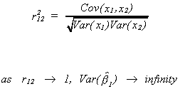
Then we can show

where

Clearly, the classic case of multicollinearity affects the precision of our estimator. Of course, in the event that x₁ and x₂ have an exact linear relationship the situation is even worse. The best that we could hope to do would be to estimate the single regression coefficient in y_i = ax_i + u_i, where a = b₁ + lb₂

Example
The model is
y_t = b₁ + b₂x_2t + b₃x_3t + b₄x_4t + u_t
y_t is import demand for France
x_2t is a dummy variable for entry into the EEC in 1960
x_3t is GDP
x_4t is gross capital formation

The results, with standard errors in parentheses, are

All t statistics are significant.
Suppose we include an additional variable; consumption.

 
The inclusion of x₅ has sopped up all the variation in y that had been previously explained by x₃. The consumption variable is almost indistinguishable from GDP. The correlation between them is .99.

Multicollinearity, Characteristic Vectors and Roots

Suppose y = xb+ u. We can find the characteristic vectors of x'x. Call them A, so A'x'xA = L,  where L is a diagonal matrix of the characteristic roots of x'x. Since A is a collection of orthogonal vectors we can write (x'x)^-1 = AL^-1A'. Now we usually write , but we can also write it in terms of the characteristic roots and vectors; .
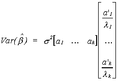
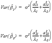
Now write A = [ a₁ a₂ ... a_k ] where a_j is a kx1 column vector corresponding to the j^th column of A. This allows us to rewrite the variance as

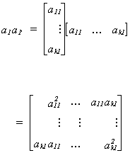
Looking at a particular product of a pair of vectors we have

a₁ is the characteristic vector in the first column of A and
a₁'(x'x)^-1a₁=l₁ so a₁ may be thought of as picking off the variance of b₁. So for a particular coefficient in the regression model

If one of the a_jl² is quite large relative to its characteristic root then we have a problem. Or, if one of the l_k is quite small then we have a problem.

Using characteristic roots and vectors there is some simple geometry to the problem.
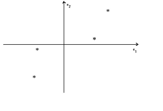
Assume that the number of observations is n=4 and the number of unknown location parameters is k=2. The scatter of observations on the indpendent variables is shown in figure 1.  Each * corresponds to the plot of an observation on x₁ and x₂

Figure 1

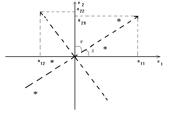
where e₁ and e₂ are the basis vectors for the space spanned by the two 4x1 vectors of observations on the independent variables. The characteristic vectors of x'x form a new basis which has the following relation to the original (see figure 2).

Figure 2

For this two variable model we have

Note and recall that the law of cosines is adjacent over hypotenuse. So cos(d) = a₁₁ is large relative to a₁₂ and cos(y)=a₂₁ is small relative to a₂₂.
Now Ax'xA' = L and x'xa_i = l_ia_i, or a_i'x'xa_i = l_i. Making a simple transformation we can rewrite this as z_i'z_i = l_i. So l_i can be thought of as the variation in the data along the i^th axis, since z_i'z_i is the explained sum of squares of the projection of the n observations onto a_i. In our diagram the data along a₁ is quite spread out, but is quite compressed along a₂, so l₁ >> l₂. Therefore, numerator and denominator in are of the same order of magnitude. However, a₂₂² is large and l₂ is small so the large size of implies that b₂ is measured with less precision.

Example:

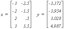
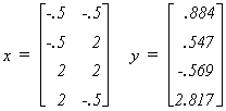
We can give some numerical flesh to the exposition. In our example we are given the following design matrix and observations on the dependent variable:



Working in the real world of empirical analysis this would be all you would know about the data generating process. Since this is an experiment designed to show you the effects of multicollinearity, the following information is also provided



This should enable you to compute the four realizations of the disturbance vector. Can you do it?
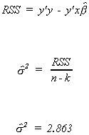
Given the data, we can calculate the least squares coefficient estimates as. Now calculate an estimate of the error variance



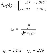
Now we have enough information to compute the variance-covariance matrix for the coefficient vector and the observed t-statistics.

The critical t for a two tail test at the 10% level with two degrees of freedom is 2.9. No coefficient is statistically different from zero, in spite of what we know to be the truth.
Recall that the characteristic roots of a matrix of full rank are all nonzero. The roots for the matrix x'x are 45.642 and 1.358. While neither is zero, the larger is 33.6 times larger than the smaller. On the basis of our earlier observations about the variance of the estimator, this is potentially a problem. The simple correlation between the two indpendent variables is .942. The characteristic vectors corresponding to the two roots are. In figure 3 these vectors and the four observations for the independent variables are plotted. The vectors are the short, perpendicular lines at about 45^o to the usual axes. These vectors form the basis for the same vector space. Notice, however, that in the a₁ dimension the data on the independent variables is not very spread out. In the a₂ dimension it is quite variable. The figure also shows the regression line of x₁ on x₂; the dashed line.

Figure 3

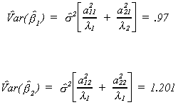
As shown above, we can calculate the coefficient variances from the characteristic roots and vectors.

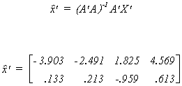
We can also use the matrix of characteristic vectors, A = [ a₁ | a₂ ] to transform the original data onto the new basis of the vector space. There are four data points, with two coordinates each. This projection is given by

If we square each term then add across the rows we get an explained sum of squares for each of the two dimensions

Notice that these sums of squares are the characteristic roots. If the data are spread out along one of the characteristic vectors then we get a large root. If the data does not show a lot of variation along one of the vectors then we get a small root.

Returning to the coefficient variances in terms of roots and vectors, we see that a large estimated variance of the coefficient estimator can result from an unfortunately large error variance. There is nothing one can do about this. There could also be a lack of variation in the data along one of the characteristic vectors. This is often characterized by data having an elliptical shape in the plane of the independent variables, rather than being scattered in a spherical or cube shape. The large estimate of the coefficient variance might also be due to unfortunate values for the elements of the characteristic vectors. The sizes of these elements are related to the rotation of the axes of the characteristic vectors relative to the original axes. The rotation is large when the data has a lot of variation in one variable, but not the other, or when the independent variables are highly correlated.
Let us repeat the example with a 'good' design matrix. This design matrix is good in the sense that the simple correlation between the independent variables is zero. The observed data is now

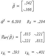
The true coefficient vector is unchanged. There has been a new draw from the N(0,2) distribution for the error vector. Applying least squares we obtain the following results


Neither coefficient is different from zero. Since the correlation between RHS variables is zero, the conventional researcher might conclude that multicollinearity is not the source of his/her bad results. On the other hand, while neither of the two variables is significant, they do explain 29% of the variation in the dependent variable. This is usually taken as evidence that there is collinearity.

The eigen values for the matrix x'x are 6.25 and 10.75. On the basis of the condition number there is no reason to suspect that collinearity is the problem. To sort out all of this, Figure 3 is repeated for the new design matrix. In figure 4 we again show the regression of x₁ on x₂, the characteristic vectors, and the data.

Figure 4
It would seem that the bad results are a result of the unfortunately large estimate of the error variance, which inflates the estimates of the variances of the coefficients.

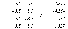
Now repeat the exercise again with another 'bad' design matrix and a new set of observed values of the dependent variable.



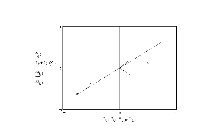
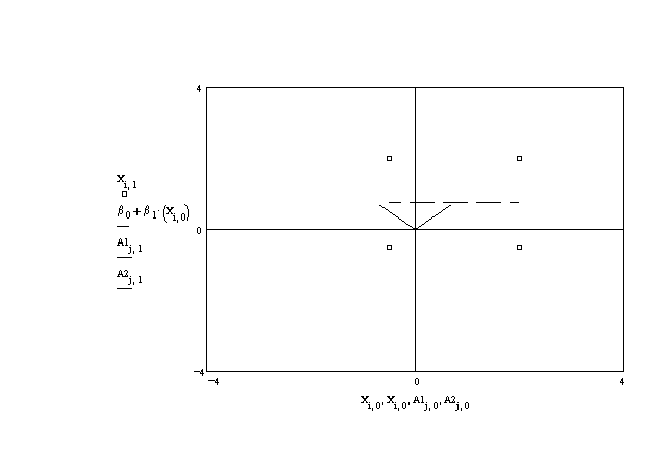
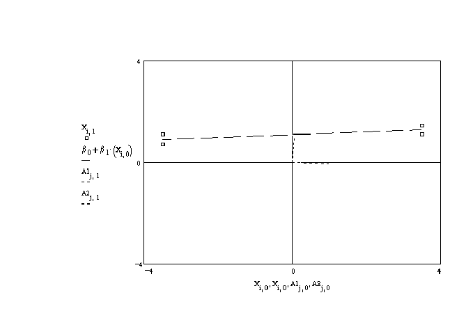
The data are plotted in figure 5 as the small boxes. The figure suggests that there is little or no relation between them; the regression line is the dashed line. The simple correlation is .70, rather high. The basis vectors corresponding to the eigen vectors of x'x lie very nearly along the original basis.


Figure 5

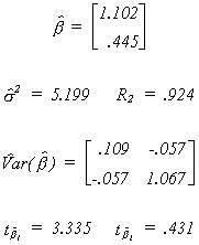
The model results are

One coefficient is now different from zero. Why isn't the other also different from zero? The characteristic roots are 49.156 and 4.856. The largest is about ten times the size of the other. This is not a small condition number, although the graph suggests that collinearity is not a problem. The problem here is that the data is rather spread out along one axis, but not the other. This ill conditioned design matrix produces a set of results which one might ascribe to multicollinearity.

Finally, we turn to the received doctrine about multicollinearity.

Consequences
1. Even in the presence of multicollinearity, OLS is BLUE and consistent.
2. Standard errors of the estimates tend to be large.
3. Large standard errors mean large confidence intervals.
4. Large standard errors mean small observed test statistics. The researcher will accept too many null hypotheses. The probability of a type II error is large.
5. Estimates of standard errors and parameters tend to be sensitive to changes in the data and the specification of the model.

Detection
1. A high F statistic or R² leads us to reject the joint hypothesis that all of the coefficients are zero, but the individual t-statistics are low.
2. High simple correlation coefficients are sufficient but not necessary for multicollinearity.
3. Farrar-Glauber suggest regressing groups of variables on a culprit. If there is collinearity then the resulting F statistic will be large.
4. One can compute the condition number. That is, the ratio of the largest to the smallest root of the matrix x'x. This may not always be useful as the standard errors of the estimates depend on the ratios of elements of the characteristic vectors to the roots.

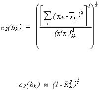
5. Leamer suggests using the magnification factor

where R_k.² is the coefficient of determination from the regression of one of the explanatory variables on all of the others.


Remediation
1. Use prior information or restrictions on the coefficients. One clever way to do this was developed by Theil and Goldberger. See, for example, Theil, Principles of Econometrics, Wiley, 1971, P 347-352.
2. Use additional data sources. This does not mean more of the same. It means pooling cross section and time series.
3. Transform the data. For example, inversion or differencing.
4. Use a principal components estimator. This involves using a weighted average of the regressors, rather than all of the regressors. The classic in this application is George Pidot, "A Principal Components Analysis of the Determinants of Local Government Fiscal Patterns", Review of Economics and Statistics, Vol. 51, 1969, P 176-188.
5. Another alternative regression technique is ridge regression. This involves putting extra weight on the main diagonal of x'x so that it produces more precise estimates. This is a biased estimator.
6. Some writers encourage dropping troublesome RHS variables. This begs the question of specification error.

Now that you've finished reading the notes, go to "Explorations in Multicollinearity."