The General Linear Model
The garden variety linear model can be written as
Y = Xb + U
A. Assumptions
1. The design matrix, n observations on each of k variables, is fixed in repeated samples of size n. This implies that X : nxk is not stochastic. Also, n > k.
2. The n x k design matrix is of full column rank. That is, the columns of the design matrix are linearly independent. The implication is that the columns of X form a basis for a k-dimension vector space.
3.a. The n-dimension disturbance vector U consists of n i.i.d. random variables such that
E(U) = 0
E(UU') = s²I_n
where s² is an unknown parameter.
Or,
b. The disturbance vector is an n-variate normal r.v.

The assumption that the design matrix be non stochastic is unnecessarily stringent. We only need assume that the disturbances and the independent variables are independent of one another.
B. Statement of the Model
Let Y be an n x 1 vector of observations on a dependent variable. For example, the crime rate in each of a number of communities at a point in time, or in one community over a number of time periods.
Let X be n observations on each of k independent variables, n>k. For example, distance of community from the urban center, relative wealth of the community, and probability of apprehension.
While Y is an n-dimensional vector, we have only k variables to explain it. This leaves us with two observations. First, we have too many equations, n, and too few unknowns, k. Second, we will need a rule for mapping the n-vector into the k-dimensional space spanned by the columns of X.
We postulate the following linear model
Y = Xb + U
where b is a k x 1 parameter vector and U is an n x 1 disturbance vector. b is not observable.

C. Least Squares Estimation of the Slope Coefficients
1. The Estimator
We wish to choose b to minimize the sum of squared deviations between the observed values of the dependent variable and the fitted values for our given data on X. That is

X_i denotes the i^th realization of the k independent variables.
In vector notation we wish to minimize, by our best guess for the unknown parameter vector, a quadratic form which we will denote by Q

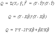
We proceed in the usual fashion by deriving the k first order conditions

Set each of the equations to zero and solve for the unknown parameters.

Note that in solving the system of equations for the k unknowns it was critical that the columns of X be linearly independent. Were they not independent it would not have been possible to construct the necessary inverse.
2. The Mean of the Estimator

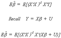
We should note several things: Expectation is a linear operator. The error term is assumed to have a mean of zero. X'X cancels with its inverse. Initially we assumed that X is non-stochastic. So

The least squares estimator is linear in Y, and by substitution it is linear in the error term. It is also unbiased.

3. The Variance of the Estimator
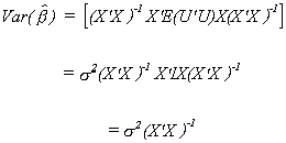
Our starting point is the definition of the variance of any random variable.

Substituting in from the expression for the mean of the parameter vector

Again, since the X are non-stochastic and expectation is a linear operator we can cut right to the heart

4. The Gauss Markov Theorem
We now come to one of the simpler and more important theorems in econometrics. The Gauss-Markov Theorem states that in the class of linear unbiased estimators the OLS estimator is efficient. By efficient we mean that estimator with the smallest variance in its class.
_{Theorem
If r(X) = k where X: nxk
E(U) = 0 E(UU')=s2I
then}

_{is BLUE.}
Proof:
We seek an estimator b^* that is a linear unbiased estimator with a smaller variance than the OLS estimator.
Let b^* = C^*Y be an arbitrary linear estimator. Since this is a linear estimator and OLS is a linear estimator we can choose C^* to be a combination of the design matrix. Namely, C^* = C + (X'X)^-1X'.
As before Y = Xb + U.

For b^* to be unbiased we must impose the restriction that CX = 0. Now from the definition of variance and using the fact that our new estimator is unbiased we have Var(b^*) = E(b^* - b)(b^* - b)'. Or, substituting in for b^*

But we already know CX = X'C' = 0 so

Since CC' must be positive semi-definite we know
Var(b^*) ³ Var()
D. Estimation of the Variance of the Error Vector
We will construct our estimator by analogy. Our assumption was that E(UU') = s²I; or, EU_i² = s² for i=1,2,..,n. It seems plausible then that we use the sum of squared residuals from our least squares estimator in the construction of an estimate of the error variance. Letting e denote the least squares residual, the sum of squared residuals is

Dividing this by n-k gives us our estimator

There is some logic to this choice of denominator. As we shall see, it gives us an unbiased estimator. Second, there are n observations and we have already used them to compute k estimates, so should be penalized accordingly. Third, because of the method of construction of the estimator of b, we can freely choose only n-k of the least squares residuals. Furthermore, the numerator has a chi-square distribution with n-k degrees of freedom.
Before taking expectations we will substitute in for Y and for the fitted values of Y.

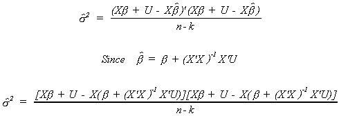
With a bit of algebra we can write this as

This is clearly a scalar. Taking the trace changes nothing, but allows us to change the order of multiplication.

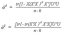
We know that EUU' = s²I. The trace of the first identity matrix is n, the second trace is k. Therefore, we conclude that

E. Maximum Likelihood Estimation
Recall that in our development of the OLS estimator we made the following assumptions:
1. E(U) = 0
2. E(UU') = s²I
3. X is fixed in repeated samples of size n
4. r(X) = k < n; X is of full column rank
and from these assumptions we can show that OLS is BLUE.
Suppose that we replace the first two assumptions by
U ~ N(0,s²I).
With this assumption we can construct the maximum likelihood estimator.
The intuition behind the maximum likelihood estimator is that knowing the distribution function that generated the data and having a sample in hand, we must pick estimates of the distribution parameters which make it most likely to have observed the particular sample. Consider the following parable: The Queen has a son in need of a spouse. She issues a proclamation stating that whosoever is able to guess the number of balls in an urn by her throne may have the son in marriage. The balls in the urn are numbered consecutively from one. Suitors are permitted to reach into the urn and withdraw a ball prior to making their guess. If the guess is incorrect then the suitor is fed to the lions. Ghislain, from Provençe, wants to take her chances. What should be her rule for construction of a maximum likelihood estimate? Suppose she reaches into the urn and withdraws a ball with the number 59 on it. Would she ever guess 100 balls in the urn? The answer is no. If there are 100 balls in the urn the probability of drawing number 59 is only 1/100. If there are 59 balls in the urn then the probability of drawing number 59 rises to 1/59.
Returning now to regression analysis, the joint density of U, the disturbance vector is

But note that U = Y - Xb. Making this substitution

Reasoning from the parable recited above, what set of b and s² will give the greatest likelihood of having observed the particular disturbance vector?
We write the likelihood function as

We wish to maximize this function by our choice of b and s². This requires setting the first derivatives of £(.) with respect to b and s² equal to zero. Since exponents are tough to deal with we will take logs. The log likelihood function is

Let us expand the last term to get

Now

Solving the first k equations for b

The last equation is

Multiply through by 2s⁴

If we use our previous convention of e denoting the fitted residuals we can write

While this is similar to our previous result, it is clear that this is not an unbiased estimator of the error variance. It is however, consistent, which we prove elsewhere in the lecture notes. Recall that we had defined consistency as

That is to say, the probability that our estimator differs from the population parameter by more than an arbitrarily small number can be driven to zero by increasing the sample size.
Since the maximum likelihood estimator is the same as the OLS estimator and U ~ N(0,s²I) we conclude

Furthermore

We previously proved that OLS is BLUE. As a result of our stronger assumption for deriving the MLE we can make a stronger statement about the behavior of . The following theorem has been provided by C.R. Rao.
_{THEOREM
If Y = Xb + U and U ~ N(0,s²I), then the maximum likelihood estimatoris the best (minimum variance) estimator in the class of unbiased estimators.}

This is a stronger result than Gauss-Markov since we have broadened our attention to include both linear unbiased and nonlinear unbiased estimators.
F.1. Hypothesis Testing
1. General Remarks
Let us assume U ~ N(0,s²I). We had adopted the notation for our model Y = Xb + U and the least squares residuals e = Y - X. The OLS estimator is = (X'X)^-1X'Y. Making the obvious substitutions allows us to write
e = Y - X(X'X)^-1X'Y
e = (I - X(X'X)^-1X')Y
e = (I - X(X'X)^-1X')(Xb + U)
e = (I - X(X'X)^-1X')Xb + (I - X(X'X)^-1X')U
The first term is zero, so e = (I - X(X'X)^-1X')U. Recall from the linear algebra chapter that (I - X(X'X)^-1X') is an idempotent matrix of order nxn. But what of its rank?
Rank(I - X(X'X)^-1X') = Rank(I) - Rank(X(X'X)^-1X')
The identity matrix is rank n. The rank of X is k so the rank of the second term is also k. So we are left with the following conclusion
e'e =U'(I - X(X'X)^-1X')'(I - X(X'X)^-1X')U
e'e = U'(I - X(X'X)^-1X')U ~ s²c²_n-k
In what follows we will adopt the following naming and notation conventions:
e'e is often called the residual sum of squares, RSS
Y'Y is often called the total sum of squares, TSS
Y'Y - e'e is the estimated or explained sum of squares, ESS
Depending on the objective, the explained sum of squares is often written in several other forms:

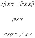
These are all found by substitution for the definition of Y and/or beta hat.
We now have sufficient machinery to test some hypotheses.
2. Student's t test
Define

In general we may wish to test the hypothesis

where

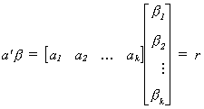
Some specific examples include the following
1. Choose a₁ = 1 , a_i = 0 for i=2,3,...,k, r=0. Then the null is that b₁ = 0.
2. Choose a_i = 1 , a_j = 0 for j ¹ i and r = 0. Then the null is that b_i = 0.
3. Choose a_i = 1 " i. Then the null is that Sb_i = r.
4. Choose a_i = 1 , a_j = -1 , all other a_l = 0. Then the null is that b_i - b_j = 0.
As a test statistic for the general form of the hypothesis test we propose

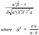
The a' and a in the denominator pick off the appropriate elements of the covariance matrix of the estimator to construct the variance of the linear combination of random variables in the null hypothesis.
It can be shown that if U ~ N(0,s²I) then under the null hypothesis

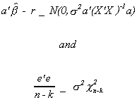
Furthermore, these two random variables are independent of one another. Therefore

3. The F test
It may be the case that we wish to do more than conduct tests of hypothesis on each of the b_i or some linear combination of them. We might want to construct a joint test involving M £ k of the model coefficients.

Let us adopt the following notation
W: denotes the complete model or the maintained hypothesis
w: denotes a simplified model, in which the parameters of the model satisfy the constraints as specified in the null hypothesis.
For instance, our maintained model might be
Y = b₁ + b₂X₂ + . . . + b_kX_k + U
and would be named W. Our simplified model might be
Y = b₁ + U
and would be named w. The implication of these two models is that quite possibly only the intercept matters. In this example we would retrieve the residual sum of squares from the regression results on the maintained and simplified model. That is,

Using the notation we have adopted so far, a typical Analysis of Variance (ANOVA) table, from standard regression routines, for the null that all of the slope coefficients are zero is

o TSS-RSS_w is the variation in Y explained by the intercept.
o RSS_w-RSS_W is the variation in Y, beyond that explained by the mean of , explained by the independent variables.
o RSS_W is the variation in Y left over after taking account of the intercept and slope parameters.
For the example we are now doing
H_o: b₂ = ... = b_k = 0
H₁: b_i ¹ 0 for some i
we would construct the test statistic

Notice that the degrees of freedom in the numerator is the number of variables restricted to zero in going from the complicated model to the simple model. If the observed F is larger than an appropriate critical F then we must conclude that one, or some, or all of the b_i i = 2,...,k are not zero.
EXAMPLE
Suppose we had the following model

and we wish to test the hypothesis

The restricted version of the model would be

To construct the test statistic first estimate W and find the sum of squared errors (RSS_W). Then estimate w and find RSS_w. Construct

F.2. Restricted least Squares
In the previous section we relied on the "restricted model" in doing both the F and t-test. Just how does one construct the restricted model estimates when the restrictions involve more than simple zero restrictions?
We have the model y = X + u with E(u X)= 0, E(u'X) = 0 and Euu'=²I. In addition we have some prior information in the form of J<k exact, independent, linear restrictions R-r=0. Previously we had chosen a best guess for using the principle of least squares. With the addition of the restrictions we must now use the method of Lagrange multipliers.


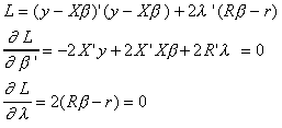
The first k first order conditions can be rearranged as follows

From the same first order conditions we can also write

Substituting r = R from the last J first order conditions we have

So the restricted least squares estimator is given by

The estimator is just a linear combination of the ordinary least squares estimator, b. That is, we need only run the unrestricted regression, then do a few computations to get the restricted estimates.
The mean of this estimator is seen to be

So the restricted least squares estimator is unbiased only when the linear restrictions are identically correct.
The variance of the estimator is found as

Doing the multiplication and exploiting the properties of idempotent matrices

Both terms in square brackets are positive definite, since they are both variances. The first term is the OLS covariance matrix, from which we are subtracting another positive definite matrix. The result is positive definite since it is a covariance matrix. Clearly then the restricted least squares estimator has a smaller variance than its unrestricted counterpart. However, this is not the end of the story. Although it has a smaller variance, the restricted estimator may be biased, so they choice of estimator is not so simple. We will revisit this question in the section which reviews hypothesis testing and model selection in multiple regression.

G. Confidence Ellipses and Intervals
1. Confidence Interval for One Parameter
Constructing a confidence interval for one parameter in a regression model is done analogously to the procedure you used for constructing confidence intervals for the mean of a random variable. Assume first that U ~ N(0,s²I_n). Then

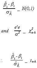
Note that

so we can write the following probability statement

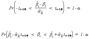
2. Confidence Ellipse for a Set of Parameters
Just as the confidence interval is the dual to the test of significance of a single parameter, the confidence ellipse is the dual to an F-test. Suppose there is a set of variables for which we wish to construct a joint confidence interval. Begin by reordering and partitioning the slope coefficients so that the M which interest us are in the top part of the coefficient vector:

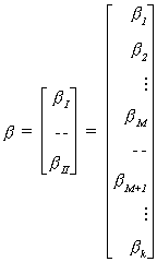
Then

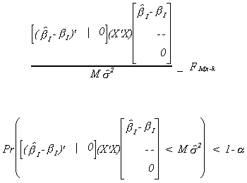
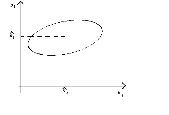
For the case where M=2 we get a result that looks like

1
The elongation and tilt of the ellipse are determined by the quadratic form (X'X). By finding the characteristic roots and vectors of X'X one can first tilt the ellipse to one of the axes then squash it into a circle. See your homework assignment from the linear algebra chapter.
H. Coefficient of Determination
Recall that we defined the coefficient of determination to be
R² = ESS/TSS
or

and noted that a serious problem with this was that for a given n we can always bring R² closer to 1 by throwing in more variables. A solution to this problem is

This is known as the adjusted R². The researcher pays a penalty for throwing in extraneous variables.
Some people use the adjusted R² as a selection criterion for additional independent variables. This is a poor practice since the adjusted R² is order sensitive. That is, if you put the variables together in a different order you may find the adjusted R² going up with the addition of X_j only a small amount under one order and a lot under another.
Some Algebraic and Geometric Insights into OLS

1. From the normal equations:

X'Xb-X'y=0
or
X'(y-Xb)=0
We recognize y-Xb as the discrepancy or residual vector. So, for every column of X we have x_k'e=0.
i. This means that the regression hyperplane passes through the origin.
ii. Since the first column of X is ordinarily a column of ones it means that .

In ii. the left hand side is the mean of the actual values and the RHS is the mean of the fitted values. They are equal, on average.

2. Projection matrices

By definition e = y-Xb
substitute for b, the least squares estimator
e=y-X(X'X)^-1X'y
e=(I_n-X(X'X)^-1X')y
e=My
We can see, from above, that MX=0. Therefore, M and X span subspaces that are orthogonal complements.

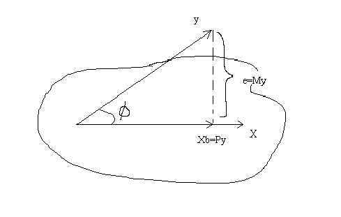
We can see that y is composed of the combination of two orthogonal components

By substitution

so P=X(X'X)^-1X' is the matrix which projects y onto the subspace spanned by X. And M=I-P is the matrix which projects y onto the orthogonal complement of X.

The rank of X is k, the rank of I_n is n. Therefore, (P)=k and the rank of M=n-k.

THEOREM (Davidson and Mackinnon, P. 11-12) Invariance
The fitted values of y and the residuals are invariant to nonsingular, linear transformations of the matrix of regressors.
Proof: Results from the invariance of the subspace spanned by X. The importance is that it doesn't really matter where we put the decimal in our RHS data if our only interest is forecasting. In fact, from a computational and rounding error standpoint, it pays to rescale the data in your model to indices whenever the units of measurement are markedly different.

3. Goodness of Fit

If we plug our best guess for the coefficients into the objective function, then the sum of squared residuals is

(y-Xb)'(y-Xb)= e'e
= (y-X(X'X)^-1X'y)'(y-X(X'X)^-1X'y)
= y'MMy
= y'My
= My ² the length of the residual vector.

Expanding the LHS of the first line

e'e=y'y-2b'X'y+b'X'Xb
for the middle term we can write
-2b'X'y = -2y'X(X'X)^-1X'y
= -2[y'X(X'X)^-1](X'X)[(X'X)^-1X'y]
so
e'e = y'y-b'X'Xb
or
y'y=b'X'Xb+e'e

So we can offer the following
b'X'Xb = (y'X(X'X)^-1X')(X(X'X)^-1X'y)
= (Py)'(Py)
= Py² , the length of the fitted vector.

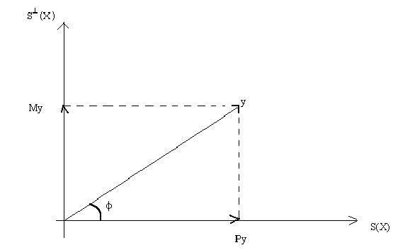
So the conclusion is

This lends itself to an interpretation of goodness of fit. If the discrepancy between y and the fitted vector is quite small then the length of the residual vector will be quite short. Or, the length of the fitted vector will be quite close to the length of y. A natural definition then is

where the subscript u denotes "uncentered", the meaning of which will become clear in a moment.
From a bit of trigonometry

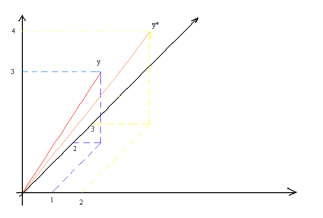
But we have a problem. Suppose we add a constant to each element in the vector y. Consider a specific example: The model is y=x₁b₁+x₂b₂+u. Our original data is
. Now . Applying our least squares estimator, b=(X'X)^-1X'y.


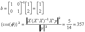
But suppose we add 1 to each observation on y so , but X is unchanged. Then .

We have raised the goodness of fit measure by the simple expedient of adding a constant to each observation on y! Note that if we multiply y by a scalar there would be no impact on the goodness of fit measure, since it merely lengthens y but does not displace it in the n-dimensional space (See the following picture).

Since x₁ and x₂ are the first two vectors in the orthonormal basis you should be able to sketch them in. Also sketch in . You can now see why the R_u² has gone up.

In the Bread and Meat exercise set you had to take logs of meat consumption. The problem was that in some cases meat consumption was zero. One suggested fix up was that you add a small number to each observation. You now can see the consequence of doing this.

To get around the problem we measure y as a deviation from its mean

and calculate


And the moral of the story is that you must always include a constant.

4. Partitioned Regression

Suppose that we are entertaining the model y = X + u, which we are able to partition as y = X₁₁ + X₂₂ + u, in which X₁ and X₂ are nxk₁ and nxk₂, respectively. The normal equations are


with some algebra
b₁ = (X₁'X₁)^-1X₁'y - (X₁'X₁)^-1X₁'X₂b₂
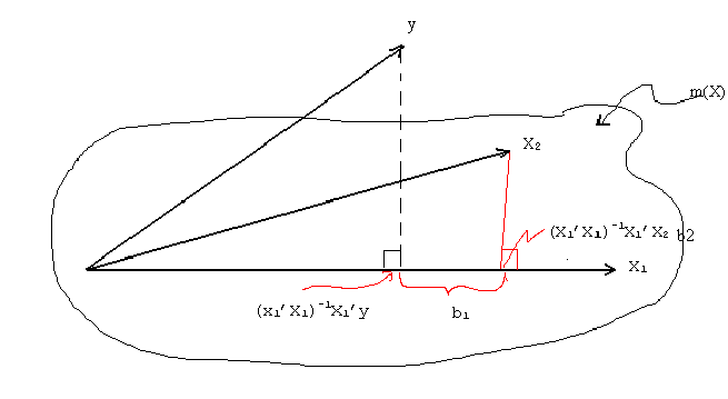
The first term on the RHS is the projection of y onto the space spanned by the columns in X₁. Looking more closely at the 2^nd term,(X₁'X₁)^-1X₁'X₂ is the projection of each of the columns of X₂ onto the space spanned by X₁. We can represent this in the following diagram:


In the figure X₁ and x₂ span a k₁+k₂ dimensional space denoted by m(X), and which looks like a lake or artist's palette.
With more algebra
b₂ = [X₂'(I-X₁'(X₁'X₁)^-1X₁')X₂]^-1 (X₂'(I-(X₁'X₁)^-1X₁'))y
To interpret this consider the following
Step 1. Regress y on X₁ alone and save the residuals to get

y = X₁₁ + u₁


and

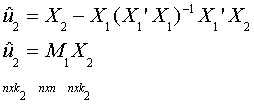
Step 2. Regress each of the columns of X₂ on the set of regressors X₁

Note the dimensions are shown. So

Step 3. Now let us run the regression model

by substitution

by idempotency

which we know to be b₂.

Another important result is that the residuals from direct estimation of the original model and the residuals at the final step of the partitioned model will be the same.

Implications:

1. The result presented in the figure is known as the Waugh-Frisch-Lovell Theorem (WFL). The main result is that it permits the "ceteris paribus" interpretation of coefficients.
2. It means detrending and deseasonalizing the the data (with dummies) first is equivalent to including a time trend and seasonal dummies on the RHS.
3. At the time of programming it can economize on computation.