I

II.A. DISCRETE RANDOM VARIABLES

1. BINOMIAL

Requirements for a random variable to be binomial:

1. The experiment consists of "n" identical trials.

2. There are only two possible outcomes for each trial.

3. The trials are independent of one another.

4. The probability of success is the same on each of the n trials.

5. The random variable is defined as the number of successes in n trials.

The binomial theorem is:

This probability function is indeed a probability distribution

a. p and 1 - p are fractions

b. the combinatorial part need not be a fraction.

you could prove to yourself P(x) 1. Also

so it satisfies the axioms of probability.

Example: We are producing a part on a machine with P(S) = .6 and P(F) = .4

Consider 3 parts chosen at random, let x = no. of good parts.

`X`	`P(X)`
`0`	`.064`
`1`	`.288`
`2`	`.432`
`3`	`.216`

Let us now consider the expected value of a binomial random variable.

Recall

Now we have a specific probability function in mind

take out np and cancel the x

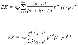
let r = x-1, m = n-1

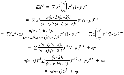
Using more slight of hand we can find the variance of a binomial random variable.

Var(X) = EX² - (EX)²

for a binomial r.v.

(EX)² = n²p²

and

The binomial is of interest to us because we could use a set of independent variables to model the probability of success. In practice we usually do this by assuming that the underlying data generating process is logistic or normal because they are more flexible.

2. POISSON

Suppose we wish to find the probability distribution of the number of auto accidents at a particular intersection during a period of 1 week.

Divide the week into n subintervals so small that at most one accident could occur in any one interval with P(accident) > 0. Define

P(1 accident in a subinterval) =p

Let be the average value of the random variable, number of accidents, observed over many intervals, say n, of the same size. Then the probability of x accidents is

It can be proved that the Poisson distribution is a limiting case of the binomial.

Example: A machine producing widgets averages 1 bad in a production run of 100 parts. p = .01.

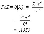
Suppose we produce n = 200. What is the probability of there being no defects? Using the binomial

Using Poisson

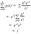
Poisson is a probability distribution satisfying the axioms of probability. We prove one of them here

MEAN OF POISSON RANDOM VARIABLE

VARIANCE

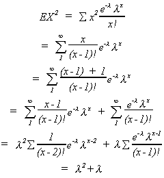
Since (EX)² = l², we know Var(X) =l.

The Poisson has many applications in economics and management science. The classic paper on Poisson regression, in which the rate parameter is modeled by a set of independent variables is Jorgensen. It has been used to model aggregate strike activity and traffic accidents.

II.B. CONTINUOUS RANDOM VARIABLES

INTRODUCTION: A continuous random variable whose domain is any real number. It can be on the open interval (-Ą,Ą) or any sub-interval.

AXIOMS

1.

2.

MEAN

VARIANCE

1. NORMAL DISTRIBUTION

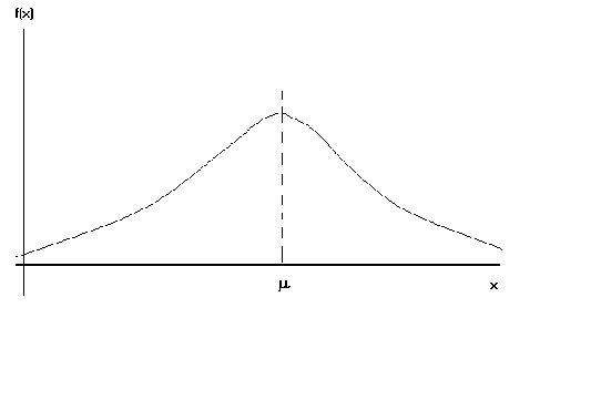
The density is given by

where = mean and = variance of the random variable X. This could be awkward to integrate by parts for every problem. Fortunately every normal random variable can be transformed into one having a given mean and variance.

Let , then

Now let

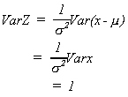
so we have transformed the normal random variable x into Z with = 0, = 1. This means we only need to know how to do one specific integration.

Note

The normal is

1. symmetric

2. asymptotic to horizontal axis.

3. is neither platy- nor leptokurtic.

Click here to see what the normal distribution looks like.

Suppose

Needless to say, this is a difficult integration. Fortunately someone has gone to the trouble of integrating and tabulating a N(0, 1) variable.

So note

we now have our question in terms of the tables.

Example: Hulk Hogan, former Olympic heavyweight wrestler, has agreed to meet a randomly selected SUMA wrestler. We know the following about such wrestlers

We also know that Hogan weighs 345 pounds. He wants to know the probability that the visiting SUMA is bigger than he

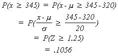
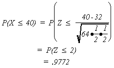
It should be noted that when n, the number of trials is large the binomial may be approximated by the normal.

Example: Flip a penny 64 times

or

2. CHI-SQUARE DISTRIBUTION

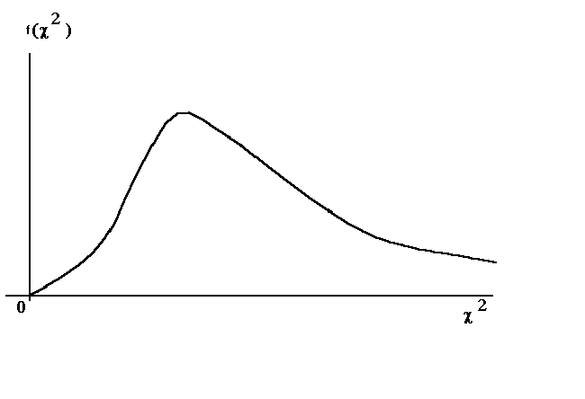
The chi square random variable is related to the normal distribution. Suppose we observe a whole bunch of normal random variables that are independent of each other. Let us select, randomly, ten

x₁, x₂, ... , x₁₀

Transform them

Square these and add them up

where = 10

1. The number of degrees of freedom determines the shape of the distribution. As it approaches a normal.

2.

3.

Example: You should be able to use a set of tables to see how these are done.

1.

2.

Suppose that we had constructed

and

Then y has a non-central chi square distribution. That is, it is more skewed than if we had used the proper construction. The non-centrality parameter is

The usual tables are for the central chi-square. In order to calculate probabilities for a non-central distribution you would have to write an approximation algorithm. Such algorithms can be found in Abramowitz and Stegun, Handbook of Mathematical Functions, Dover Publications, New York, 1970.

II.C. CHEBYSHEV'S INEQUILITY AND LAWS OF LARGE NUMBERS

This section will be your first introduction to asymptotic theory. You will find much more in a later section of the lecture notes.

Let us first state "An Inequality"

Let x be a non negative random variable and t be a positive number. We wish to know the probability that the random variable will exceed t. We integrate the probability density from t to infinity.

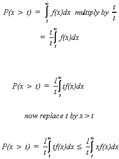
Let us add on another piece to the right side

so or

CHEBYSHEV'S INEQUALITY

Let x be a random variable with E(X) = and Var(X) = then

Proof:

As in the previous theorem we have a non negative random variable and a positive number so that

since we can write

WEAK LAW OF LARGE NUMBERS

Let x₁, x₂, ... be independent and identically distributed random variables with mean and variance . Then for each positive number we can write

Proof: Using Chebyshev we can say that

We know, using the rules of expectations,

Then

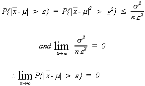
We have just shown that the sample mean is a consistent estimator of the population mean.

CENTRAL LIMIT THEOREM

Suppose x₁, x₂, ... , x_n are iid random variables.

Let

Then mean of S_n is and

Now transform S_n to get

which has a mean of zero and a variance of one. Now,

In layman's terms, the theorem states the following:

The distribution of the means of random samples taken from a population having mean and finite variance approaches the normal distribution with mean and variance as the sample size, say n, becomes large.

This will prove to be very useful. Its importance lies in the fact that regardless of the distribution of the random variable x, the distribution of will be normal. This allows us to not only engage in hypothesis testing, but parametric hypothesis testing.