SPECIFICATION PROBLEMS

A. Omission of a Relevant Variable
Suppose that the true model is

but through some error in judgement we estimate the parameters of the model

That is we incorrectly omit the k^th independent variable. What are the consequences of having omitted the k^th variable? Define

The estimate from the incorrectly specified model is

To check for bias we will substitute in for y

Let us take a closer look at P. Begin with the product of the design matrix with the last column omitted and the correct design matrix.

Substitute back into the estimator

Now consider the second term. Except for b_k, it looks like an OLS estimator resulting from regressing x_k on the remaining independent variables. That is,

So the bias of the least squares estimator for the omitted variables model is

The LS estimator is biased except when either

1. b_k = 0
or
2. for all i. If this is the case then x_k is linearly independent of all the other columns of x.
or
3. Suppose x_k is uncorrelated with the other columns of x, then the slopes are unbiased but the intercept is biased unless the mean of x_k is also zero.

B. Inclusion of an Irrelevant Variable
No problem, Mon. If an irrelevant variable is included, then in expectation it takes the value of zero and has no impact on the correctly included variables. Nor, in expectation, does it change the efficiency of least squares. However, we don't live in a perfect long run world. Consequently, since including more variables necessarily reduces the residual sum of squares, the estimate of the coefficient variance will be smaller. In practice we may find ourselves rejecting too many null hypotheses.

1. Functional Form
   

1. Functions Linear in Parameters
Almost every modern econometrics textbook presents material on nonlinear estimation. This seems to me to be much ado about nothing. To begin with, the small sample properties of these estimators are not well understood. At best we can say something asymptotically. With OLS we can say a great deal both in large samples and in small samples.
Secondly, the nonlinear estimation routines are computationally burdensome. They rely on a hill climbing algorithm that either minimizes the sum of squared errors or maximizes the likelihood function. Most software packages offer at least two algorithms for this. In the fine print they always remind the user to choose starting values carefully. There is usually a caveat that choice of functional form is important for avoiding local minima or maxima.
A third problem is that economic data is often very flat. That is, for the observed data, the ascent on the likelihood function may not be very steep. As a result the algorithm may wander around on likelihood function until the number of iterations is used up. The closing round estimates may be quite different depending on the chosen starting values for the model parameters.
The final reason that non-linear estimation is a great deal of noise to little effect is that there are other useful alternatives. Not only are there other alternatives, but in most cases we would be quite justified in using the alternative. We know from the Weierstrasse Theorem that we can approximate, to any desired degree, any continuous and continuously differentiable function with a polynomial of sufficiently high degree.
There are exceptions to these comments. The most notable one is in time series analysis. If ARIMA models are to be estimated by maximum likelihood then nonlinear routines are the only way to go.

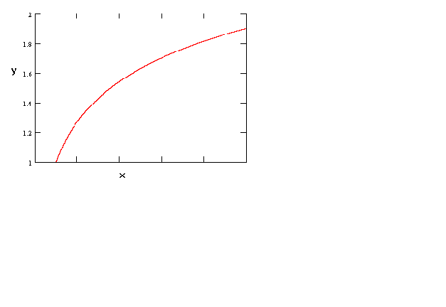
Figure 1

y = a + b ln(x)



As a first example consider the above figure. This is just the semi-log function .

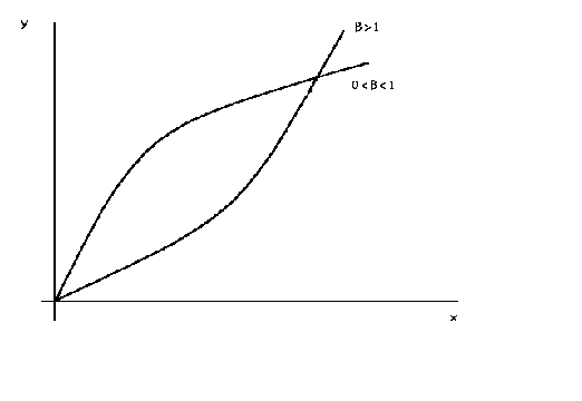
Figure 2

ln(y) = a + b ln(x)
The above example is the log-log function. Whether the curve is concave or convex depends on the size of b. If there were another right hand side variable or two then the function would be the familiar Cobb-Douglas function. By simply changing the sign on b we can get a curve that looks like an indifference curve or an isoquant, as in the following figure. By altering the magnitude of b it is possible, in the context of indifference curves, to show a relatively stronger preference for one good or the other.
Figure 3

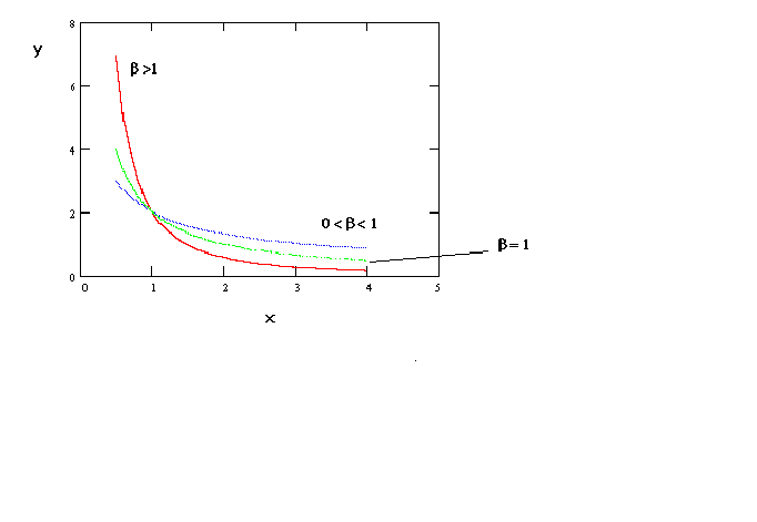
ln(y) = a - b ln(x)
If one uses the inverse of the independent variable then one gets a curve as in figure 4.

Figure 4 y = a + b (1/x)
The curve is convex and approaches an asymptote from above.
This might be useful for estimating a money demand function. Elsewhere in this chapter you will encounter the Box-Cox transformation. This is the usual model for money demand. As you will see, it is an analytically cumbersome technique.

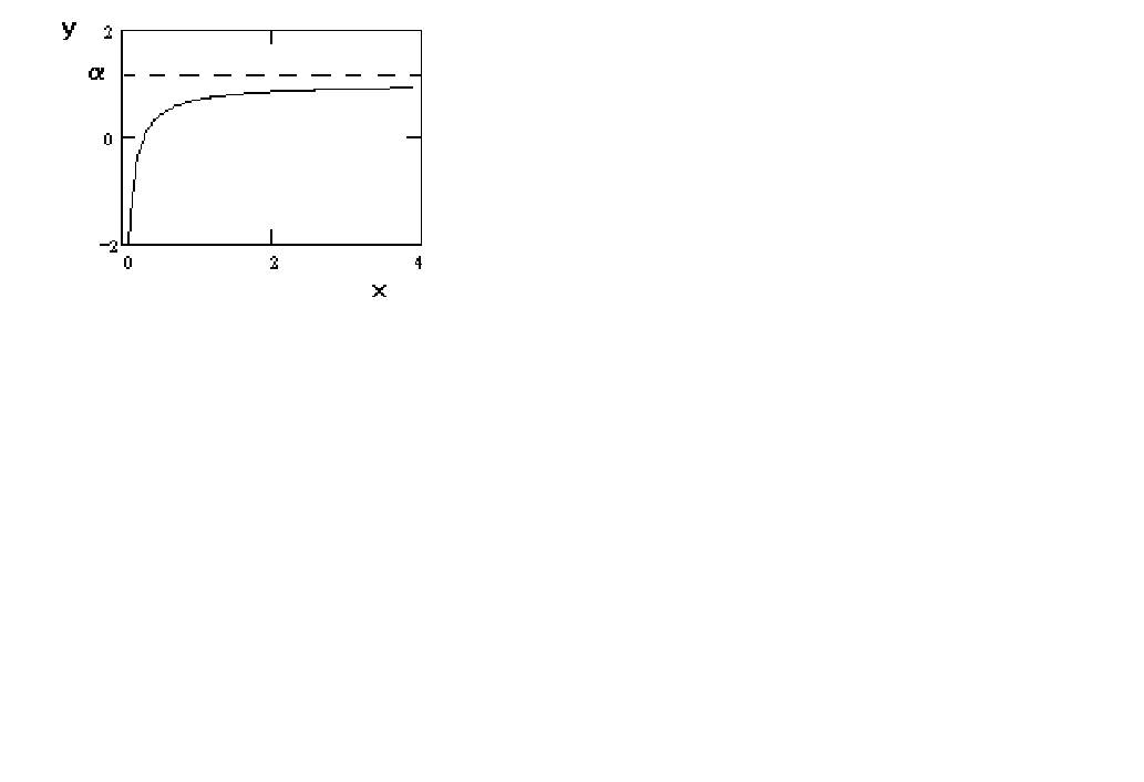
Figure 5 y = a - b (1/x)

In figure 5 we just change the sign on the coefficient in the 'money demand' function. The result is that it is concave and approaches the asymptote from below.
In figure 6 we can produce a sigmoidal shape by proper choice of the parameters. For example, a production function might have this shape if over the relevant range of output there is not a negative marginal product. For most problems in economics this seems quite plausible.

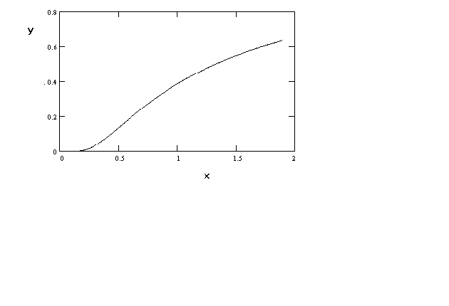
Figure 6 ln(y) = a + b (1/x)

In Figure 7 we have a parabola.

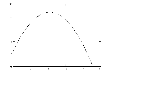
Figure 7 y = a + bx + gx²
By suitable choice of parameters we could flip it over and have an average cost curve.
Finally, although the coefficients have been chosen to exaggerate the shape, a cubic function can be chosen to create a production function or cost function that is well behaved.

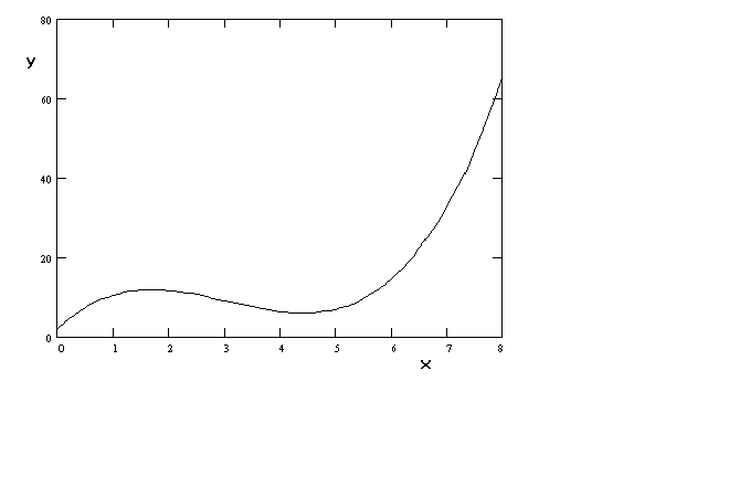
Figure 8 y = a+ bx + gx² + dx³

The curves in figures 7 and 8 do present their own challenges at the time of estimation. It is often found that when the independent variable is entered on the right hand side in polynomial form the problem of multicollinearity rears its ugly head. This can be overcome in part, for example, by estimating an average cost curve instead of a total cost curve. So doing entails dropping, say, the cube term from the function. Another solution is found in the use of orthogonal polynomials. See F.A. Graybill, An Introduction to Linear Statistical Models, McGraw-Hill, 1961, Pp. 172-182.

2. The Box-Cox Transformation
We begin with the observation that if we define f(z) as follows

then for

The last line is found by applying L'Hopital's Rule. Given the flexibility of this transformation it is suggested that the classical linear regression model be written as

The least squares estimates are

(i)

One would proceed by any one of several methods. The easiest would be a Taylor Series expansion of (i). Use the OLS estimates of b as a starting point then conduct a grid search over .

D. Dummy Variables and Splines
The models discussed in this section are very closely related to the earlier work on restrictions and tests of hypothesis.
1. Dummy Variables
Case 1
Suppose we have earnings data on workers who can be divided as

We also have a continuous variable called x, perhaps age, so the full model is

Using OLS to estimate all the parameters we can then discuss the effects of membership in particular groups. For example, suppose that we want to predict the earnings of a non-union, uneducated male. The predicted earnings, conditional on x, are

If we have a union member, educated, single female then the predicted earnings are

The idea is that each group has its own independent intercept, but all have the same slope on x.

Case 2

We could use dummies to model different slopes for different groups. Consider an example with just two groups.

We have the model with one RHS variable

If the individual is a male then we get

For a female

The female differs from the male in both intercept and slope. In this case, in which all of the RHS variables receive the dummy variable treatment, we could apply OLS to the individual subsets of data and get the same results. In an instance where some slope is common then we want to apply OLS to the pooled data.

Case 3

Suppose we have a quarterly time series. Instead of setting up a dummy variable for three of the four quarters as in

we get lazy and construct a variable that takes the following form

Then, blundering along, we estimate the three parameters of

The results by quarter are

First Quarter

Second Quarter

Third Quarter

Fourth Quarter

The effect of creating this funny RHS variable, S, to account for the seasonal differences is to make the quarter-to-quarter shift the same between any pair of quarters. Is this plausible? You will also see this kind of careless construction in cross sections in which firms in industry 1 have a variable with a value of 1, firms in industry 2 have a variable with a value of 2 and so on.

2. Splines

Splines have their origin in architecture and engineering. In those disciplines a fair curve needs to be fitted to a set of points and a french curve just won't do the trick. Instead they use a flexible rubber edge which can be bent to any curve. It is held in place by weights called ducks. A point where the curve changes its shape is called a knot.
Return to the earlier example in which there were two groups of wage earners differing in slope and intercept, but the slope did not change as the worker aged. The estimated model would appear


But suppose, in a new study, we think that the rate of change of wages should depend on age. The model needs to be modified so that the slope coefficient differs over prespecified intervals. There is also the stipulation that the resulting curve be continuous at the points where there is a change in slope. The new model should look like

The function parameters to be estimated are

Wage = a^o + b^o Age if Age < 18

Wage = a¹ + b¹ Age if 18 £ Age < 22

Wage = a² + b² Age if 22 £ Age

To implement this in a form that satisfies the continuity constraint and which is amenable to least squares let us define

The full model will be

The three slopes are

In order to ensure that the segments meet at the join points we must impose the following restrictions

This linear spline can be generalized in a couple of ways. First, the segments between the knots can be polynomials. Second, there can be more RHS variables with interactions. This has the effect of fitting planes with different gradients over the space spanned by the RHS variables.

Testing Non-nested Hypotheses

Suppose we have two alternative models that we are entertaining and wish to choose between them on statistical grounds. That is,

The models differ in the set of right hand side variables.
Define

Then the estimates of the error variances from the two specifications are

Suppose that model (1) is the truth. Then our estimate of the error variance of model two can be rewritten as

Upon taking expectations the middle term will drop out.

We can use a trick from our earlier examination of the unbiasedness of the error variance estimator. Namely, we will take the trace.

Substituting back

We can see that in expectation the estimated error variance of the incorrect model exceeds the error variance of the correct model. The question is whether we can detect this difference statistically. To do this we construct the statistic

What is the probability limit of this test statistic? By Slutsky's theorem we know that the probability limit of a function of a random variable is equal to the function of the probability limit of the random variable.

from (3) we can see that the numerator and the denominator are equal in the limit, so plim C₁₂ = 0.

and we can use the test statistic

There is a serious drawback to this test. Namely, it is not symmetric. We began by stating that (1) was the correct model and constructed a test statistic on this basis. If we begin by stating that (2) is the correct model and construct the test statistic then it is quite possible that we could reach a different conclusion. This is not the only time we encounter a conflict of criteria. It happens in the use of the LM, LR and Wald tests in finite samples. We also noted that using R² as a rule for variable inclusion is a bad idea since order matters.