A Brief Introduction to Modern Time Series
Definition A
time series is a random function xt of an argument t in a set T. In other
words, a time series is a family of random variables ..., xt-1, xt,
xt+1, ... corresponding to all elements in the set T, where T is supposed to be
a denumerable, infinite set.
Definition An observed time series {xt | t e To Ė T} is regarded as a part of one realization of a random function xt. An infinite set of possible realizations which might have been observed is called an ensemble.
To put things more rigorously, the time series (or random function) is a real function x(w,t) of the two variables w and t, where wÎW and tÎT. If we fix the value of w, we have a real function x(t|w) of the time t, which is a realization of the time series. If we fix the value of t, then we have a random variable x(w|t). For a given point in time there is a probability distribution over x. Thus a random function x(w,t) can be regarded as either a family of random variables or as a family of realizations.
Definition We define the
distribution function of the random variable w given t0
as P{x(w|to) Ģ x} = (x). Similarly we can define the joint distribution
for n random variables
The points which distinguish time series analysis from ordinary statistical analyses
are the following
(1) The dependency among observations at different chronological points in time plays an
essential role. In other words, the order of observations is important. In ordinary
statistical analysis it is assumed that the observations are mutually independent.
(2) The domain of t is infinite.
(3) We have to make an inference from one realization. The realization of the random
variable can be observed only once at each point in time. In multivariate analysis we have
many observations on a finite number of variables. This critical difference necessitates
the assumption of stationarity.
Definition The random
function xt is said to be strictly stationary if all the finite dimensional
distribution functions defining xt remain the same even if the whole group of
points t1, t2, ..., tn is shifted along the time axis.
That is, if
for any integers t1, t2, ..., tn and k. Graphically,
one could picture the realization of a strictly stationary series as having not only the
same level in two different intervals, but also the same distribution function, right down
to the parameters which define it.
The assumption of stationarity makes our lives simpler and less costly. Without
stationarity we would have to sample the process frequently at each time point in order to
build up a characterization of the distribution functions in the earlier definition.
Stationarity means that we can confine our attention to a few of the simplest numerical
functions, i.e., the moments of the distributions. The central moments are given by
Definition (i) The mean
value of the time series {xt} is

i.e., the first order moment.
(ii) The autocovariance function of {xt} is
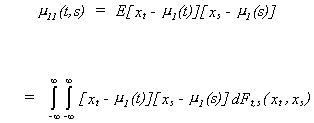
i.e., the second moment about the mean. If t=s then you have the variance of xt.
We will useto denote the autocovariance of a
stationary series, where k denotes the difference between t and s.
(iii) The autocorrelation function (ACF) of {xt} is
We will useto denote the autocorrelation of a
stationary series, where k denotes the difference between t and s.
(iv) The partial autocorrelation (PACF), fkk, is the correlation between zt
and zt+k after removing their mutual linear dependence on
the intervening variables zt+1, zt+2,
..., z t+k-1.
One simple way to compute the partial autocorrelation between zt and zt+k
is to run the two regressions
then compute the correlation between the two residual vectors. Or, after measuring the variables as deviations from their means, the partial autocorrelation can be found as the LS regression coefficient on zt in the model
10 |
where the dot over the variable indicates that it is measured as a
deviation from its mean.
(v) The Yule-Walker equations provide an important relationship
between the partial autocorrelations and the autocorrelations. Multiply both sides of
equation 10 by z t+k-j and take expectations. This
operation gives us the following difference equation in the autocovariances
or, in terms of the autocorrelations
This seemingly simple representation is really a powerful result. Namely, for j=1,2,
..., k we can write the full system of equations, known as the Yule-Walker equations,
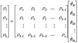
From linear algebra you know that the matrix of r's is of
full rank. Therefore it is possible to apply Cramer's rule successively for k=1,2,... to
solve the system for the partial autocorrelations. The first three are


We have three important results on strictly stationary series.
First, if {xt} is strictly stationary and E{xt}2
< Ĩ then
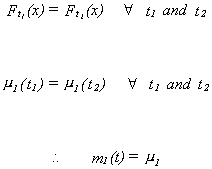
The implication is that we can use any finite realization of the sequence to estimate
the mean.
Second, if {xt} is strictly stationary and E{xt}2
< Ĩ then
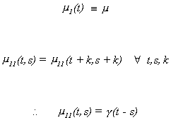
The implication is that the autocovariance depends only on the difference between t and
s, not their chronological point in time. We could use any pair of intervals in the
computation of the autocovariance as long as the time between them was constant. And we
can use any finite realization of the data to estimate the autocovariances.
Thirdly, the autocorrelation function in the case of strict stationarity
is given by
The implication is that the autocorrelation depends only on the difference between t
and s as well, and again they can be estimated by any finite realization of the data.
If our goal is to estimate parameters which are descriptive of the possible realizations
of the time series, then perhaps strict stationarity is too restrictive. For example, if
the mean and covariances of xt are constant and independent of the
chronological point in time, then perhaps it is not important to us that the distribution
function be the same for different time intervals.
Definition
A random function is stationary in the wide sense (or weakly stationary, or
stationary in Khinchin's sense, or covariance stationary) if m
1(t) šm and m11(t,s) = .
Strict stationarity does not in itself imply weak stationarity. Weak stationarity does not
imply strict stationarity. Strict stationarity with E{xt}2 < Ĩ implies weak
stationarity.
Ergodic theorems are concerned with the question of the necessary and sufficient
conditions for making inference from a single realization of a time series. Basically it
boils down to assuming weak stationarity.
Theorem If {xt} is weakly
stationary with mean m and covariance function , then
That is, for any given e > 0 and h
> 0 there exists some number To such that
for all T > To, if and only if
This necessary and sufficient condition is that the autocovariances die out, in which
case the sample mean is a consistent estimator for the population mean.
Corollary If {xt} is weakly
stationary with E{xt+kxt}2 < Ĩ
for any t, and E{xt+kxtxt+s+kxt+s} is
independent of t for any integer s, then
if and only if where
A consequence of the corollary is the assumption that xtxt+k is
weakly stationary. The Ergodic Theorem is no more than a law of large numbers when the
observations are correlated.
One might ask at this point about the practical implications of stationarity. The most common application of use of time series techniques is in modelling macroeconomic data, both theoretic and atheoretic. As an example of the former, one might have a multiplier- accelerator model. For the model to be stationary, the parameters must have certain values. A test of the model is then to collect the relevant data and estimate the parameters. If the estimates are not consistent with stationarity, then one must rethink either the theoretical model or the statisticla model, or both.
We now have enough machinery to begin to talk about the modeling of univariate time
series data. There are four steps in the process.
1. building models from theoretical and/or experiential knowledge
2. identifying models based on the data (observed series)
3. fitting the models (estimating the parameters of the model(s))
4. checking the model
If in the fourth step we are not satisfied we return to step one. The process is iterative
until further checking and respecification yields no further improvement in results.
Diagrammatically

Definition Some simple
operations include the following:
The backshift operator Bxt = xt-1
The forward operator Fxt = xt+1
The difference operator Ņ = 1 - B
Ņxt = xt - xt-1
The difference operator behaves in a fashion consistent with the constant in an
infinite series. That is, its inverse is the limit of an infinite sum. Namely, Ņ-1 = (1-B)-1 = 1/(1-B) = 1+B+B2+
...
The integrate operator S = Ņ -1
Since it is the inverse of the difference operator, the integrate operator serves to
construct the sum .
MODEL BUILDING
In this section we offer a brief review of the most common sort of time series models. On
the basis of one's knowledge of the data generating process one picks a class of models
for identification and estimation from the possibilities which follow.
Autoregressive Models
Definition Suppose that
Ext = m is independent of t. A model such as
with the characteristics is called the
autoregressive model of order p, AR(p).
Definition If a time
dependent variable (stochastic process) {xt} satisfiesthen {xt} is said to satisfy the Markov property. On the LHS
the expectation is conditioned on the infinite history of xt. On the RHS it is
conditioned on only part of the history. From the definitions, an AR(p) model is seen to
satisfy the Markov property.
Using the backshift operator we can write our AR model as
Theorem A necessary and
sufficient condition for the AR(p) model to be stationary is that all of the roots of the
polynomial
lie outside the unit circle.
Example 1
Consider the AR(1) 
The only root of 1 - f1B = 0 is B = 1/f1. The condition for stationarity requires that .
If then the observed series will appear very
frenetic. E.g., consider
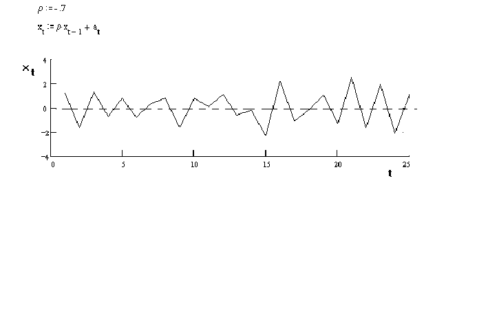
in which the white noise term has a normal distribution with a zero mean and a variance
of one. The observations switch sign with almost every observation.
If, on the other hand, then the observed series
will be much smoother.
E.g.
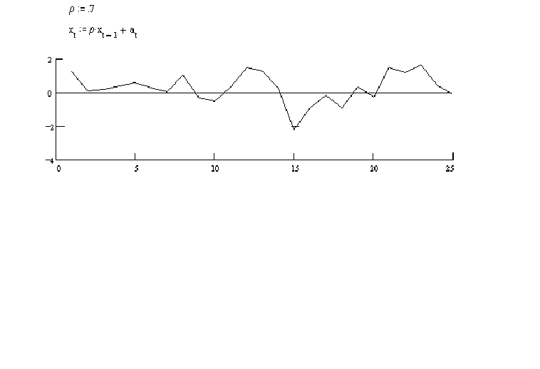
In this series an observation tends to be above 0 if its predecessor was above zero.
The variance of et is se2
for all t. The variance of xt, when it has zero mean, is given by
Since the series is stationary we can write .
Hence,
The autocovariance function of an AR(1) series is, supposing without loss of generality m=0
To see what this looks like in terms of the AR parameters we will make use of the fact
that we can write xt as follows
Multiplying by xt-k and taking expectations
Note that the autocovariances die out as k grows. The autocorrelation function is the
autocovariance divided by the variance of the white noise term. Or,.
Using the earlier Yule-Walker formulae for the partial autocorrelations we have

For an AR(1) the autocorrelations die out exponentially and the partial autocorrelations
exhibit a spike at one lag and are zero thereafter.
Example 2
Consider the AR(2) The associated
polynomial in the lag operator is
The roots could be found using the quadratic formula. The roots are
Whenthe roots are real and as a consequence the
series will decline exponentially in response to a shock. When
the roots are complex and the series will appear as a
damped sign wave.
The stationarity theorem imposes the following conditions on the AR coefficients
The autocovariance for an AR(2) process, with zero mean, is
Dividing through by the variance of xt gives the autocorrelation function
Since
we
can write
Similarly for the second and third autocorrelations


The other autocorrelations are solved for recursively. Their pattern is governed by the
roots of the second order linear difference equation
If the roots are real then the autocorrelations will decline exponentially. When the
roots are complex the autocorrelations will appear as a damped sine wave.
Using the Yule-Walker equations, the partial autocorrelations are
Again, the autocorrelations die out slowly. The partial autocorrelation on the other
hand is quite distinctive. It has spikes at one and two lags and is zero thereafter.
Theorem If xt is
a stationary AR(p) process then it can be equivalently written as a linear filter
model. That is, the polynomial in the backshift operator can be inverted and the AR(p)
written as a moving average of infinite order instead.
Example
Suppose zt is an AR(1) process with zero mean; . What is true for the current period must also be true for prior
periods. Thus by recursive substitution we can write
Square both sides and take expectations
the right hand side vanishes as k Ū Ĩ
since ―f― < 1. Therefore the sum
converges to zt in quadratic mean. We can rewrite the AR(p) model as a linear
filter
that we know to be stationary.
The Autocorrelation Function
and Partial Autocorrelation Generally
Suppose that a stationary series zt with mean zero is known to be
autoregressive. The autocorrelation function of an AR(p) is found by taking expectations
of
and dividing through by the variance of zt
This tells us thatrk is a linear combination
of the previous autocorrelations. We can use this in applying Cramer's rule to (i) in
solving for fkk. In particular we can see that this
linear dependence will cause fkk = 0 for k > p.
This distinctive feature of autoregressive series will be very useful when it comes to
identification of an unknown series.
If you have either MathCAD or MathCAD Explorer
then you can experiment interactivley with some fo the AR(p)
ideas presented here.
Moving Average Models
Consider a dynamic model in which the series of interest depends only on some part
of the history of the white noise term. Diagrammatically this might be represented as
Definition Suppose at
is an uncorrelated sequence of i.i.d. random variables with zero mean and finite variance.
Then a moving average process of order q, MA(q), is given by
Theorem: A moving average
process is always stationary.
Proof: Rather than start with a general proof we will do it for a
specific case. Suppose that zt is MA(1). Then . Of course, at has zero mean and finite variance. The mean
of zt is always zero. The autocovariances will be given by
You can see that the mean of the random variable does not depend on time in any way. You
can also see that the autocovariance depends only on the offset s, not on where in the
series we start. We can prove the same result more generally by starting with , which has the alternate moving average
representation
. Consider first the variance of
zt.
By recursive substitution you can show that this is equal to
The sum we know to be a convergent series so the variance is finite and is independent of
time. The covariances are, for example,
You can also see that the auto covariances depend only on the relative points in time, not
the chronological point in time. Our conclusion from all this is that an MA(Ĩ) process is stationary.
For the general MA(q) process the autocorrelation function is given by
The partial autocorrelation function will die out smoothly. You can see this by inverting
the process to get an AR( ) process.
If you have either MathCAD or MathCAD Explorer
then you can experiment interactively with some of the MA(q)
ideas presented here.
Mixed Autoregressive - Moving Average Models
Definition Suppose at
is an uncorrelated sequence of i.i.d. random variables with zero mean and finite variance.
Then an autoregressive, moving average process of order (p,q), ARMA(p,q), is given by
The roots of the autoregressive operator must all lie outside the unit circle. The number
of unknowns is p+q+2. The p and q are obvious. The 2 includes the level of the process, m, and the variance of the white noise term, sa2.
Suppose that we combine our AR and MA representations so that the model is
(1) |
and the coefficients are normalized so that bo = 1. Then this representation is
called an ARMA(p,q) if the roots of (1) all lie outside the unit circle.
Suppose that the yt are measured as deviations from the mean so we can drop ao,
then the autocovariance function is derived from
if j>q then the MA terms drop out in expectation to give
![]()
That is, the autocovariance function looks like a typical AR for lags after q; they die
out smoothly after q, but we cannot say how 1,2,…,q will look.
We can also examine the PACF for this class of model. The model can be written as
![]()
We can write this as a MA(inf) process
![]()
which suggests that the PACF's die out slowly. With some arithmetic we could show that
this happens only after the first p spikes contributed by the AR part.
Empirical Law In actuality, a stationary time series may well be
represented by p Ģ 2 and q Ģ 2. If
your business is to provide a good approximation to reality and goodness of fit is your
criterion then a prodigal model is preferred. If your interest is predictive efficiency
then the parsimonious model is preferred.
Experiment with the ARMA ideas presented above with
a MathCAD worksheet.
Autoregressive Integrate Moving Average Models
MA filter AR filter Integrate filter

Sometimes the process, or series, we are trying to model is not stationary in levels.
But it might be stationary in, say, first differences. That is, in its original form the
autocovariances for the series might not be independent of the chronological point in
time. However, if we construct a new series which is the first differences of the original
series, this new series satisfies the definition of stationarity. This is often the case
with economic data which is highly trended.
Definition Suppose that zt
is not stationary, but zt - zt-1 satisfies the definition of
stationarity. Also, at, the white noise term has finite mean and variance. We can write
the model as
![]()
This is named an ARIMA(p,d,q) model. p identifies the order of the AR operator, d
identifies the power on Ņ, q identifies the order of the MA
operator.
If the roots of f(B)Ņ lie outside
the unit circle then we can rewrite the ARIMA(p,d,q) as a linear filter. I.e., it can be
written as an MA(Ĩ). We reserve the discussion of the
detection of unit roots for another part of the lecture notes.
Transfer Function Models
Consider a dynamic system with xt as an input series and yt as an
output series. Diagrammatically we have
These models are a discrete analogy of linear differential equations. We suppose the
following relation
![]()
where b indicates a pure delay. Recall that Ņ = (1-B).
Making this substitution the model can be written

If the coefficient polynomial on yt can be inverted then the model can be
written as

V(B) is known as the impulse response function. We will come across this terminology
again in our later discussion of vector autoregressive , cointegration and error
correction models.
MODEL IDENTIFICATION
Having decided on a class of models, one must now identify the order of the
processes generating the data. That is, one must make best guesses as to the order of the
AR and MA processes driving the stationary series. A stationary series is completely
characterized by its mean and autocovariances. For analytical reasons we usually work with
the autocorrelations and partial autocorrelations. These two basic tools have unique
patterns for stationary AR and MA processes. One could compute sample estimates of the
autocorrelation and partial autocorrelation functions and compare them to tabulated
results for standard models.
Definitions
Sample Mean
![]()
Sample Autocovariance Function
![]()
Sample Autocorrelation Function
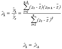
The sample partial autocorrelations will be
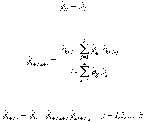
Using the autocorrelations and partial autocorrelations is quite simple in principle.
Suppose that we have a series zt, with zero mean, which is AR(1). If we were to
run the regression of zt+2 on zt+1 and zt we would expect
to find that the coefficient on zt was not different from zero since this
partial autocorrelation ought to be zero. On the other hand, the autocorrelations for this
series ought to be decreasing exponentially for increasing lags (see the AR(1) example
above).
Suppose that the series is really a moving average. The autocorrelation should be zero
everywhere but at the first lag. The partial autocorrelation ought to die out
exponentially.
Even from our very cursory romp through the basics of time series analysis it is apparent
that there is a duality between AR and MA processes. This duality may be summarized in the
following table.
| AR(p) | MA(q) | ARMA(p,q) | |
| The stationary AR(p) f(B)zt = at can be represented as an MA of infinite order. | The invertible MA(q) zt = q (B)at can be represented as an infinite order AR. | Can be represented as either an AR() or MA(), conditional on roots. | |
| Autocorrelation | rk Ū 0 but r đ 0 from f(B)=0. That is, the spikes in the correlogram decrease exp onentially. | rk = 0 for k ģ q+1. There are spikes until lag q. |
Autocorrelations die out smoothly after q lags. |
| Partial autocorrelation | fkk = 0 for k ģ p+1. There are spikes in the correlogram at lags 1 through p. |
fkk Ū 0 but fkk đ 0 from q(B)=0. The spikes die out exponentially | PACF's die out smoothly after p lags |
| Stationarity | All roots of f(B)=0 lie outside the unit circle. | No restriction. | |
| Invertibility |
No restriction. |
All roots of q (B)=0 lie outside the unit circle. |
Diagrams of the theoretical correlograms for AR and MA processes can be found in
Hoff(1983, Pps. 59-71) or Wei(1990, Pp. 32-66). The correlograms for a stationary ARMA are
somewhat more problematic. The autocorrelations show an irregular pattern of spikes
through lag q, then the remaining pattern is the same as that for an AR process. The
partial autocorrelations are irregular through lag p, then the PACs decay exponentially as
in an MA process.