 , is an estimator for the population mean. An estimator is a random variable since it is a rule based on random variables.
By population we mean any well defined collection of subjects that is exhaustive of the issue to be studied.Trying to collect data on every member of the defined population would be impossibly expensive so we use samples in order to infer something about the population.
A random sample is a set of observations drawn with replacement from the population on variables of interest.
An estimator is a rule for assigning using the sample data to estimate a population parameter. The sample mean, , is an estimator for the population mean. An estimator is a random variable since it is a rule based on random variables.
An estimate is the specific numerical value taken by the estimator when the data is plugged into the rule. An estimate is not a random variable.
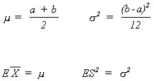
1. Unbiasedness An estimator is said to be unbiased if its expected value is equal to the population parameter for which it is an estimator.
, is an unbiased estimator of the population mean. , is an unbiased estimator of the population varaince.
2. Efficiency is a relative concept based on the variances of alternative estimators. The efficient estimator is the one with the smallest variance. In the class of linear unbiased estimators the sample mean has the smallest variance of any other such linear unbiased estimator. The result about the sample mean is proved in the Gauss-Markov Theorem.
3. Suffiency: We say that an estimator is sufficient if it uses all the sample information. The sample mean is a sufficient statistic, but the sample median is not.
4. Consistency An estimator is said to be consistent if the probability that is differs from the population parameter by more than a little bit diminishes as the sample size increases. Consistency is a large sample property.
The CLT is a special result of the law of large numbers. From the central limit theorem we know that the distribution of the sample mean approaches the normal as the sample size increases.
Probability distributions are characterized by parameters. For example, the normal distributionis characterized by the mean and the variance. The uniform distribution on the interval [a,b] is defined by the lower bound a and the upper bound b, which can be shown to be functions of the distribution's mean and variance. So, if in the functional relationships between 'a' and 'b' and the mean a varaince we substitute in the sample mean and the sample variance then we can get estimates of 'a' and 'b'. This approach is known as the method of moments.
A maximum likelihood estimator is that estimator for the population parameter which makes it most likely to have observed the sample that we actually found.
The Least Squares Estimator, abbreviated OLS, is a rule that minimizes the sum of squared differences between the sample observations and our guess for the population parameter of interest.
The sample mean and the sample variance have very desirable properties as estimators. However, the probability that an estimate is identically equal to the parameter that we are trying to estimate is zero. To overcome this problem we construct an interval around the point estimate that we have in hand. The method, or rule, that we use to construct such intervals is done so that we know the proportion of such intervals that contain the parameter of interest, although we don't know which constructed intervals contain the parameter.
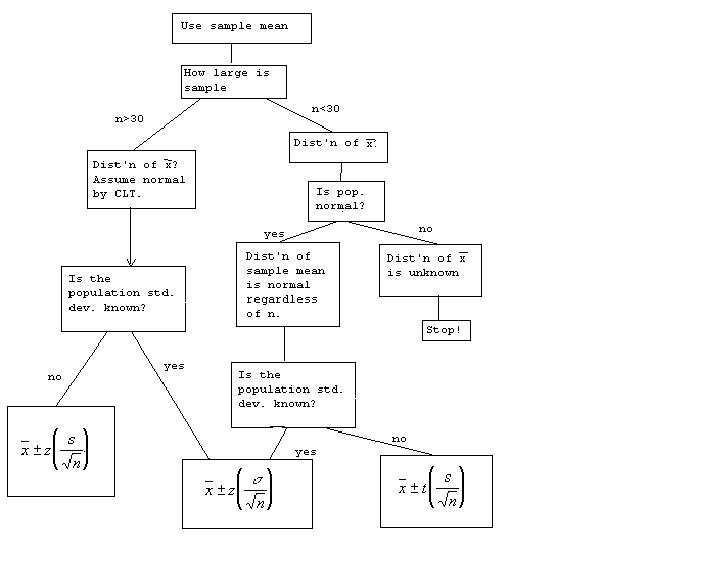
Confidence intervals for a mean:
1. Small sample, population variance known, and population distribution known to be normal:
![]()
2. Small sample, population variance unknown, population distribution known to be normal:
![]()
There is more to the story so a flow chart might help:
Confidence interval for a variance:
A test of hypothesis is the dual to the problem of constructing a confidence interval.
The null (what we believe to be true and hope isn't) and alternate hypothesis.
Type I and Type II errors. The level of the test and the power of the test.
Statistical significance and signficance in the sense of numerical magnitude.