The data for this homework consists of monthly data for the period 1981 through 1989, for a total of 108 observations. The data is for California. The dataset is traffic2.wf1. There is also a data description file.

1. During what month and year did California's seatbelt law take effect?
   
   January 1986
   
   
2. Is California's a primary or a secondary seatbelt law? You will have to look this up on the WWW.
   
   Primary
   
   
3. When did the highway speed limit increase to 65 MPH?
   
   May 1987
   
   
4. Regress the variable log(totacc) on a time trend ('t' in the dataset) and 11 monthly dummies.
   
   
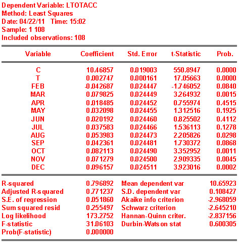
   1. Would you say that there is seasonality in total accidents? Yes
      
      How do you know? Since we are in the business of hypothesis testing we should bring these skills to bear here. The coefficient on FEB is negative and statistically different from zero. The coefficients on MAR, AUG, SEP, OCT, NOV, DEC are all positive and statistically different from zero. On the basis of the observed t-statistics, FEB must be different from the other 6 months listed. Also, the six just listed are different from APR, MAY, JUN and JUL which are zero in a statistical sense. To see whether any pair from the list of 6 are different from one another we would do simple t-tests. For example, we might consider SEP and OCT. t=(.082113-.042361)/sqrt(.000599+.000600-2*.000301)=1.6269
      
      
   2. What is the meaning of the coefficient on the time trend?
      
      Each month during the period under consideration there is a 0.2% increase in accidents.
      
      
5. Add to the regression from part 4. the variables wkend, unem, spdlaw and beltlaw.
   
   
   
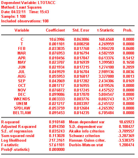
   1. Does the coefficient on unem make sense in terms of sign and magnitude? This could be argued either way. The sign is negative and significant. As the unemployment rate rises the number of accidents goes down. One could plausibly argue that when unemployment rises there is less income to buy gas and less time spent in the car. Since less time is spent driving, there will be fewer accidents. On the other hand, if one is not working then one has more time to go crusing around in one's car: more time in the car results in more car accidents.
      
      
   2. Are the coefficient estimates for spdlaw and beltlaw what you expected? Why? The coefficients are significantly negative and positive, respectively. It is a little surprising that accidents have gone down with the higher speed limit. The greater one's speed, the less time to react to an emergency situation, and therefore one would expect to see more accidnts, not fewer. On the other hand, one might argue that people drive more carefully when travelling at higher speeds. The belt law could also be interpreted either. As more people wear seatbelts they engage in more risky driving behavior in the mistaken belief that they are 'safe.' Or, once in the habit of buckling up, people are more aware of the risk of driving and are therefore more careful. Or, the intent of the seat belt law was to reduce serious injuries and fatalities once an accident has occurred, therefore one might not expect to see any change in accidents.
      
      
6. Repeat part 4., but use log(prcfat), which is pecent of accidents that result in a fatality, instead of log(totacc).
   
   
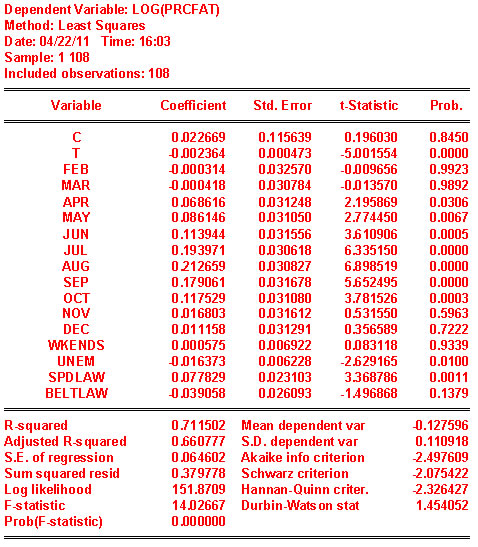
   Do your conclusions regarding seasonality and time trend change?
   
   The sign on the time trend has reversed sign. As time goes by the percent of crashes involving a fatality is decreasing. There is still seasonality in the data based on the signs and significance of the monthly dummies.The SPDLAW and BELTLAW coefficients have reversed sign and now make more intuitive sense.
   
   
7. Go back to the model of with log(totacc) on the left hand side and the time trend, seasonal dummies, wkend, unem, spdlaw and bltlaw on the RHS. Save the residuals by entering the command series res01=resid in the command window, the big white field at the top of the workfile space. Now run the regression res01_t = b₀ + b₁ res01_t-1 + v_t. At the 5% level test the null hypothesis that the coefficient on res01_t-1 is different from zero. From the results table shown below we can see that the coefficient on the lagged residual (b₁= 0.356, t=3.92, p-value = .0002) is different from zero at the 5% level.
   
   
   
8. For the original model of part 7., in the estimation dialogue box of EVIEWS add the term AR(1) and estimate the model coefficients.
   
   
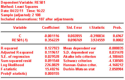
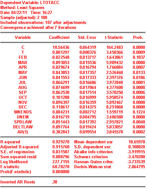
   Is the estimate of the coefficient on AR(1) the same as the coefficient on res01_t-1 of part 7?
   
   In the table the coefficient on AR(1) is 0.3828. This is somewhat larger than the estimate of the same parameter based directly on the OLS residuals.
   
   If there is a difference, how do you account for the difference? There are two explanations for the difference. First, the RHS variables may not be strictly exogenous, as called for implementing the auxiliary regression in part 7. Second, in your answer to part 7 involved losing an observation. As Wooldridge explains, there is a correction that can be implemented to restore the intitial observation.