Asymptotic Theory, Order in Probability
and Laws of Large Numbers
Notation
W is the set of all possible outcomes, or the
sample space. For example, in flipping two coins the sample space consists of {H1
H2, H1 T2, T1 H2, T1 T2},
where the subscripts are an index for the differentiable coins.
w is a particular outcome. For example, H1 H2 in the coin toss experiment.
x(w) is a function that assigns a numerical result to the outcome w. For example, it might be the number of heads in two coin tosses.
{xi(w)}i=1,2,...,T is a sequence of random variables which assigns, e.g., the proportion of heads in i tosses of a fair coin. Other examples include the sample mean or variance, or a regression coefficient.
Convergence Almost Surely
Consider the sequence x1(w), x2(w), ..., xj(w), ..., xT(w), which is the sample mean computed from a sample of size j.
Suppose E Xj(w) = m. We
know intuitively that for large enough T the sample mean approaches the population mean.
That is, by choosing a large T we can make
arbitrarily small, say less than e. This property of the random
sequnce can be written
. There are a large
number of outcomes or sequences for which this inequality remains true. Let us denote them
To illustrate how the set A is constructed we offer the following mind construct. Line
up a sequence of barrels from here to the North Pole. The barrel closest to us is filled
with random sequences of size one from which we can construct a sample mean. The next
barrel is filled with random sequences of size two from which we can construct sample
means. The next barrel is filled with random sequences of size three from which we can
construct sample means. And so on all the way to the North Pole, and beyond. If you draw a
random sequence from the barrel closest to you it is quite likely that the mean will
differ from the population mean by more than e. On the other
hand, if you draw a sequence from the barrel closest to the North Pole, a very large
sequence, it is very likely that the sample mean will be within e
of the population mean. If the sequence you drew and its associated random variable, the
sample mean, falls close to the population mean then it belongs to the set A.
Now ask yourself, what is the probability of drawing a sequence from the barrel closest to
the North Pole, or beyond, and getting a sample mean that qualifies the sequence for
membership in A? Or, similarly, what proportion of the sample space belongs to A? Or, what
is the probability of the union of the sets in A? The answer is
or
The evaluation of this probability provides our first definition.
DEFINITION Convergence Almost Surely
xt(w) converges almost surely to m if
we write this as
If xt(w) is a vector random variable then we change the norm to
Euclidean distance
Convergence in Probability
Now let us consider and pose
the question
Suppose we consider the sample mean problem again and look at
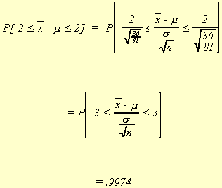
The normally distributed random variable w has a mean of 10
and a variance of 36. Suppose we initially use a sample of size nine and choose e to be 2. Then,
Suppose now we increase the sample size to 81.

We see that as the sample size is allowed to get large, the probability that the sample mean differs from the population mean gets smaller. Therefore, we arrive at the following definition.
DEFINITION Convergence in Probability
A sequence xT(w) converges in probability to m if the probability of can be made arbitrarily small for a large enough T. That is
we write .
Note the important difference from the concept of convergence almost surely. For
convergence in probability, each of the sets of events w,
has arbitrarily small probability, whereas
in convergence almost surely it was the union of the sets of events.
Theorem
If then
.
Proof:
Define . If
then for To we know
and we can say that the probability of one set of events is less than the
probability of the union of all such sets
.
Therefore
The converse is not necessarily true. However, a subset of any sequence which is convergent in probability will converge almost surely.
DEFINITION
If where k is a constant then k is
termed the probability limit of xT(w) and we denote
it as plim(xT(w)) = k.
SLUTSKY'S THEOREM
If g(x) is a continuous function then plim(g(xT)) = g(plim(xT)).
Although we state Slutsky's Theorem without proof, we note that it is used to prove that
estimators are consistent.
DEFINITION
Suppose xT(w) is used to estimate the
parameter q. If plim(xT(w))
= q then the estimator is said to be consistent.
The notion of consistency can be seen in the following diagram:
As can be seen in the diagram, increasing the sample size tightens the distribution of
the sample mean about the true mean. By choosing a large enough sample size we can make
the probability that differs from
by some derisory amount arbitrarily small.
DEFINITION
{xt(w)} converges in rth moment to
the random variable x if
(1) E[xtr] exists for all r
(2) E[xr] exists
and if .
DEFINITION
When r = 2 we refer to the above limit as convergence in quadratic mean. It is
written as .
THEOREM
This theorem is proved using Chebyshev's Inequality. When x is a constant then this is a specific form of the weak law of large numbers, and convergence in quadratic mean is a sufficient condition to prove consistency.
DEFINITION
The sequence of functions {FT} converges to the funciton F if and only
if for all x in the domain of F and for every e > 0 there
exists a To such that . This is denoted FT
® F.
DEFINITION
The sequence of random variables {xT} with corresponding distribution
functions {FT(x)} is said to converge in distribution (converge in law) to the
random variable x with distribution function F(x) if and only if FT ® F at all continuity points of F. We write either .
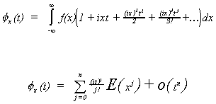
DEFINITION: Characteristic Function
Suppose x is a random variable with density function f(x), then its characteristic
function is
The relationship between the characteristic function and moments about the origin is
We will use this definition in a later proof of a law of large numbers.
THEOREM
Suppose that f(t), continuous at 0, is the
characteristic function of F(x). Let {xT} be a sequence of random variables
with characteristic functions fT(t). Then if and only if
.
Summary of Convergence Concepts
Review of Order in Probability: O and o
We will need to do some expansions in order to proceed with our asymptotic work. You may recall from your calculus course that when doing a Taylor series expansion there is always a remainder. In our work the remainder might turn out to be a nuisance. In order to justify dropping the remainder term we have to have a rule for determining and indicating how large the term is that has been dropped.
DEFINITION
Let {at} and {bt} be sequences of real variables and positive
real variables, respectively. The at
is of smaller order than bt, denoted
by at = o(bt),
if
DEFINITION
Let {at} and {bt} be sequences of real variables and positive
real variables, respectively. Then at is at most of order bt,
denoted by at = O(bt), if there exists a positive number M
such that
for all t.
Examples
(1) Consider the sequence an = 4 + n - 3n2 and the sequence bn
= n2.
The sequence is bounded by M = +3, so an
= O(n2), or an is at most of order n2.
(2) Again an = 4 + n - 3n2 and now bn = n3.
The ratio an/bn goes to zero as n ® Ą. So an is of smaller order than n3.
DEFINITION
Let {yt} be a sequence of random variables and {at} be
sequence of nonstochastic, positive real numbers. Then yt is of smaller order
in probability than at, denoted by yt = op(at)
if .
DEFINITION
Let {yt} be a sequence of random variables and {at} be
sequence of nonstochastic, positive real numbers. Then yt is at most of order
in probability at, denoted by yt = Op(at)
if for every e > 0 there is a positve M such that .
Examples
(1) Assume xt ~ N(0,s2) and consider
the sequence yt = xt/t. It should be obvious that Eyt = 0
and Var(yt) = (1/t2)s2 and we
can see that so plim(yt) = 0.
Therefore xt is of smaller order in probability than t.
(2) Assume xt ~ N(m,s2)
and consider the sequence. From a version
of the central limit theorem we know
from which we conclude that .
Central Limit Theorems
THEOREM
Let {xt} be a sequence of iid rv's with E(xt) = m and Var(xt) = s2.
Then where
.
Proof:
Let then
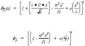
. The characteristic function of
will be given by
The underlined portion is nothing more than . Continuing to substitute in from the definition
53
*
NOTE:

A Taylor series approximation at t=0 gives

Making use of this observation, and E(x-m) = 0 and E(x-m)2 = s2,
we have

expanding by the binomial theorem we get

The summation drops out as t ® Ą
since 
which we all know to be the characteristic function for the N(0,1)!
LINDBERG-FELLER THEOREM
Let {xk} be a sequence of independent rv's with finite means and
variances. Let {ak} be a sequence of constants. Define 
if and only
if
This condition states that no term in the sequence is very important.
Uses of Lindberg-Feller:
(1) can be used to show that in large samples the distribution of sample moments is
approximately normal. That is
(2) can also be used to show that functions of the sample moments converge in
distribution to the normal.
where mj' is the jth
population moment about the origin,
mh' is the hth sample moment about the origin,
g(.) is a continuous, differentiable function.
THEOREM: Asymptotic Results for the Standard Linear Model
Consider y = x b + u with E(u|x) = 0, Var(u|x) = s2I, and n-1x'x { Qkxk. Then 1)
2) if the ui are iid then
3)
Proof:
1) We know E(i - ui) = 0 and 
. So
and by
Chebyshev's inequality
and we showed in a
previous theorem that convergence in probability is sufficient for convergence in law.
2) now premultiply by Q
for the rest of the proof consider each row of
x'u and proceed as in our previous proof of a special C.L.T.
3) follows from the above.