I. DESCRIPTIVE STATISTICS AND PROBABILITY
A. POPULATION PARAMETERS & SAMPLE STATS
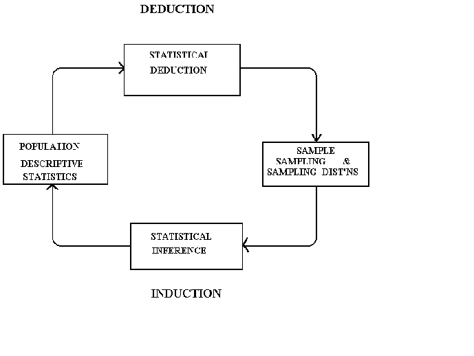
The first 5 sections of the outline may be summarized in the following diagram.
Deduction: inference by reasoning from the general to the particular.
Example: Suppose we know the average G.P.A. of all students at Temple was 2.64. If we
took a random sample of 100 we could be fairly confident in saying that the sample mean
would be near 2.64.
Induction: the process of discovering explanations for a set of particular facts by
estimating the weight of observational evidence in favor of a particular proposition.
Example: We have been told that the mean GPA at Temple is 3.0. We collect a sample from 25 students in order to test that proposition.
Population: is the set of all values under consideration, all pertinent data, the set
of all relevant values.
When an entire population is observable we will never make an incorrect decision. We
are not always able to take a census, hence the need for inferential statisics.
Example: We wish to determine the mean lifetime of 100-watt Westinghouse light bulbs so
that we may include a guarantee with the bulbs. Lifetime testing is destructive so we
clearly cannot test the entire population. But if we take a sample we may be able to infer
something about the population, at far less cost.
There are certain characteristics of a population that are referred to as parameters.
Typical examples are:
Measures of central tendency: mean, median, mode
Measures of dispersion: variance, standard deviation, range
These population parameters are knowable, although not necessarily by us.
In a similar fashion, there are characteristics of a sample that are referred to as sample statistics.
Examples:
Measures of central tendency: sample mean
Measures of dispersion: sample standard deviation, sample variance
MEASURES OF CENTRAL TENDENCY
Mode is a measure of central tendency determined by frequency. That observation
which occurs most frequently is the mode.
Median is a measure of central tendency that depends on the number of
observations. If the data is arranged in ascending order, the median is that value with
50% of the observations below and 50% above it.
While these two measures are interesting, they are difficult to deal with in a statistical sense. The median is known as an order statistic, as are the minimum and maximum in a sample. A related topic is the distribution of extreme value statistics. Consequently, we will spend little time with them. Extreme value statistics are important to people who study auctions and those who model discrete choice.
Of greatest interest and importance to beginning econometrics students among
the measures of central tendency is
the mean.
Mean, or average, or arithmetic mean measures the center of mass. As a result it
depends on the magnitude of the data points. It is merely the sum of the observations
divided by the number of observations.
Example: Suppose we had a seesaw and three people. The people are arranged along the
seesaw according to their weight, i.e., the lightest is at one end, the heaviest at the
other , while the third person is in between according to his weight.  We wish to know where to put the fulcrum so
that the seesaw is just balanced. The average weight is given by
Therefore, if we set the fulcrum at 156.66 the seesaw will just balance.
More generally, suppose that a population consists of N individuals or objects. Also, let xi represent the characteristic of interest. The population mean is given by

Note that we have used a Greek letter, mu, to denote this particular parameter. It is
convention that Greek letters denote population parameters.
Suppose that instead of observing the entire population we observed a sample of size n. Then the sample mean is given by

There are three things to note:
1. The symbol for the sample mean is a roman letter. It is convention to let letters from the roman alphabet represent sample statistics.
2. The number of elements in the population is represented by the upper case letter N. The number of observations in the sample is represented by the lower case letter n. Again, convention.
3. Also, note that the value of , the
sample mean, depends on the particular sample drawn. That is, every time we draw a new
sample the value of
will change. Thus,
is a random variable.
MEASURES OF DISPERSION
Range is the absolute value of the difference between the lowest and highest values
1. distorted by extreme values
2. uses only two observations, so some information is being omitted.
Deviation: we could consider the deviation of each observation from the mean. If
there are a large number of observations this is a bit cumbersome.
To add them up is a logical idea, but
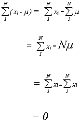
so the sum of deviations is not of much use.
Another possibility is the sum of absolute deviations, i.e.,
This is reasonable but is analytically very cumbersome. This measure does see
some use in methods of robust estimation of.
In regression analysis it would be known as the minimum absolute deviation (MAD) or linear
programming estimator.
This brings us to standard deviation and variance.
As a solution to the problem of the sum of deviations we shall first square each deviation then add them all up. Dividing by the number of observations gives us the average squared deviation. We denote this measure as the population variance, found from
Note that we have followed the conventions mentioned above. The greek sigma represents
variance, and N is the number of elements in the population.
What does the variance do for you? Recall that the mean is the center of mass. A
measure of dispersion is meant to indicate to what extent the mass is spread out. The
variance tells you exactly this. The more spead out, the greater the variance. In
classical mechanics this is also known as the moment of inertia. You can check this in
your physics or calculus text.
Example: Suppose we have two securities, IBM and ECC, two imaginary companies. They have the same mean rate of return; that being 7.5%. Without further information we would not know which one to invest in. But suppose someone provided you with the following two graphs
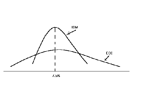
Clearly, the variance of rate of return for ECC is far greater than that for IBM.
Note that the units in the variance are squared. To make this a bit more tractable we
sometimes take the square root of the variance to get the standard deviation.
That is

Suppose that instead of observing the entire population we only observed a sample, of
size n.
Recall that the sample mean is
The sample variance is given by
Note that we have again followed convention; using a roman letter to denote a sample
statistic and a lower case letter to denote sample size.
Also note the denominator of the sample variance. Instead of dividing by the sample
size we divide by n-1. This is because we have already used the sample information to
calculate the sample mean.
The sample standard deviation is simply the square root of the sample variance

As a parenthetical note, the mean is generally called the first moment. The variance is
the second moment about the mean. The third moment about the mean determines the symmetry,
or lack of it, of the distribution. The fourth moment determines kurtosis. If a
distribution is squashed, like a plateau it is platykurtic. If it is peaked then it is
leptokurtic.
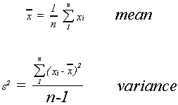
To recapitulate, we have the following population parameters
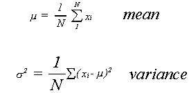
and sample statistics
I.B. SET THEORY AND PROBABILITY
We begin with three definitions of probability.
CLASSICAL: the probability of an event is the ratio of the number of ways an event can
occur to the total number of outcomes when each outcome is equally likely. An EVENT is the
outcome of an experiment.
let s = # of ways of getting A
f = # of ways A cannot occur
If we define success as picking an ace from a deck then
RELATIVE FREQUENCY
let n be the number of successes, i.e., the occurrence of A
m be the number of trials
Asthe ratio of
i.e.,
SUBJECTIVE
Degree of rational belief.
The probability of an event occurring is what you feel it to be. This is closely akin
to the notion of a prior probability in Bayesian analysis.
SOME DEFINITIONS
Consider an experiment with N possible outcomes. The set of outcomes in called the sample
space.
An event is a subset of the sample space, call the event A.
The probability of an event "A" is the number of events in "A"
divided by the number of elements in the sample space.
Example: Flip two coins. The possible outcomes are
{HH, HT, TH, TT} = sample space
Example: Choose a card at random from a fair deck. What is the probability of a face
card or a heart
A = face or heart
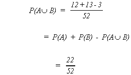
there are 13 hearts and 12 face cards, but 3 of the hearts are face cards
SET THEORY
The (set or event) C consists of the set of all points x such that x lies between zero and infinity.
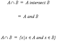
The set C consists of all points x such that x is in both A and B.
This is an example of the null set.
COMPLEMENT OF AN EVENT
The complement of an event A is denoted by .
Let S be the sample space, of which A is a subset i.e., then

Using a Venn diagram

is the shaded portion.
Using set notation
Example:

MUTUALLY EXCLUSIVE EVENTS
If A and B are mutually exclusive events then the occurrence of one precludes the
occurrence of the other.
Example: 1. on a coin flip H and T are mutually exclusive
2. on the roll of a die the events "roll a 1" and "roll a 3" are
mutually exclusive.
MUTUALLY EXCLUSIVE AND COLLECTIVELY EXHAUSTIVE
If A and B are mutually exclusive they cannot both occur at the same time. If they are
collectively exhaustive then they contain, between them, all possible outcomes in the
sample space.
Example: 1. On a coin flip H and T are mutually exclusive and collectively exhaustive.
2. "Roll a 1" and "Roll a 3" are mutually exclusive but not
collectively exhaustive.
INTERSECTION
Let X represent the points of a sample space S.
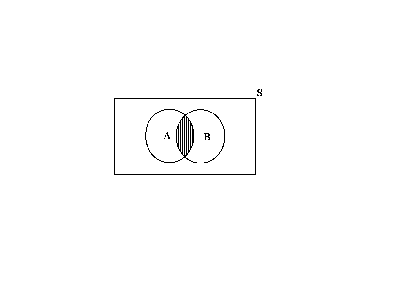
Let A and B represent two subsets of this sample space
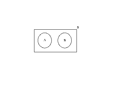
Suppose A and B do not have any points in common, i.e., they are mutually exclusive,
We can extend the idea of intersection to more than two sets.
UNION OF TWO EVENTS
The set of points that are in either or both of two events

COMPLEMENTARITY AND CONDITIONAL PROBABILITY
COMPLEMENTS
Let the sample space contain N sample points and event A contain "a" of these points. Then from our previous definition
consists of (N - a) points, so

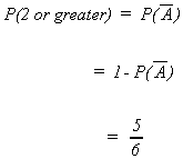
Example: Define event A as rolling a single die and getting a one. As a result, we
define as rolling a 2, 3, 4, 5 or 6
Now we ask the probability of rolling a 2 or greater
CONDITIONAL PROBABILITY
Consider the type of question such that we are interested in the occurrence of one
event given that another has occurred
In set notation
since we know B has occurred we need not worry about all of S
Our sample space is only the points in B and A�B is the set of
points common to both A and B
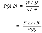
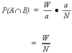
Suppose that there are N points in the sample space, "b" points in B and
"a" in the set A. Also, let there be W points in common between A and B.
The relative frequency of A�B can be determined from
and using our definition of probability
also
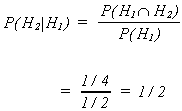
Example: Compute the probability of H on the second toss of fair coin given H on the
first toss.
S = {H1H2, H1T2, T1H2,
T1T2}
Example: Let A be the event 2 is drawn
B be the event � is drawn
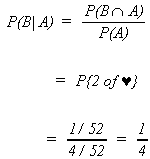
Note that in both of these examples the two events are independent.
MULTIPLICATION RULE

INDEPENDENCE
If A and B are independent then the fact that one has occurred has no bearing on whether
or not the other occurs.
Example:
The first flip of the coin has no bearing on the outcome of the second flip.
Example: let A be the event a 2 is drawn
let B be the event a � is drawn
P(B) = 1/4
P(A) = 1/13
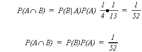
There is a special multiplication rule for independent events.
ADDITION RULE
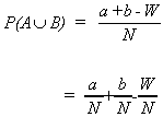
Example: Choose a card at random
A = face card
B = heart
Suppose two events are mutually exclusive, i.e.,

then
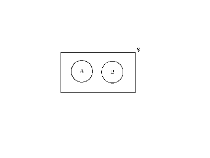
Since sets A and B don't overlap we don't have to subtract for double counting.
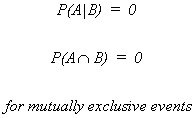
Question: Can two events be both mutually exclusive and independent?

but
BAYES RULE
Suppose we have the events A,B.
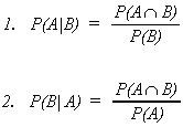
Upon rearranging 1 and 2,

equating these two gives
rearranging
Example: There are three chests in a room. Each chest has two drawers each containing a
single coin
G |
G |
S |
||
G |
S |
S |
||
I |
II |
III |
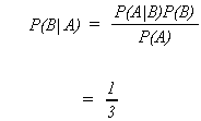
An individual staggers into the darkened room, opens a drawer, grabs a coin and
staggers out. In the light it is observed that he has a gold coin. What is the probability
that he got it from chest II?
A = gold coin
B = chest II
BAYES RULE MORE GENERALLY
Suppose we have the disjoint events
B1, B2, ..., Bn
and that
That is
B1 |
B2 |
B3 |
B4 |
||
|
|||||
|
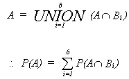
now
so
or
MARGINAL PROABABILITY
We can arrange much of our information into a table
The probabilities on the edges of the table are marginal probabilities.
II. RANDOM VARIABLES AND PROBABILITY FUNCTIONS
Definition: A random variable X is a function X:S � R
or
A random variable takes a possible outcome and assigns a number to it.
Example: Flip a coin five times, let X be the number of heads in five tosses.
X = { 0, 1, 2, 3, 4, 5}
Definition: A probability distribution assigns probabilities to all possible outcomes
of an experiment.
Example: The experiment is five flips of a coin, the random variable counts the number
of heads.
X |
P(X) |
0 |
.03125 |
1 |
.15625 |
2 |
.31250 |
3 |
.31250 |
4 |
.12625 |
5 |
.03125 |
| 1.00000 |
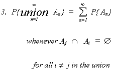
If we were to do more examples we would surmise the following axioms of probability

A third, less obvious axiom is
B. EXPECTATION
We are now prepared to introduce the notion of mathematical expectation. We begin the
development with an example.
Example: Flip two coins. For each head that appears you receive $2 from your rich
uncle. For each tail you pay him $1. The outcomes of the experiment are
X = amount you receive |
|
HH |
4 |
HT |
1 |
TH |
1 |
TT |
-2 |
As an astute player you should be interested in the probability of a particular
outcome.
X |
P(X = x) |
$4 |
1/4 |
$1 |
1/2 |
-$2 |
1/4 |
After explaining the above game, your uncle asks how much you are willing to pay in
order to play.
You are not interested in your expected winnings on any given pair of throws. We could
repeat the experiment an infinite number of times and calculate the average payoff per
trial. There is an easier way to determine this average than flipping coins for the rest
of our lives.
Expected value is merely a weighted average. The weights are the probabilities that an
outcome will occur.
Think of how we would calculate the mean if we were to flip a large number of pairs of
coins.
We would use the following:
where xi is our winning of the ith type and fi is the
number of times that outcome occurred in N trials.
But note that fi/N is nothing more than a probability when .
Since our probability distribution has already letit seems reasonable to use
for calculation of our expected winnings.
For the coin game
X |
P(X = x) |
X P(X) |
4 |
1/4 |
1 |
1 |
1/2 |
1/2 |
-2 |
1/4 |
-1/2 |
so
Our long run average winnings will be $1 per toss. We would never pay more than that to play.
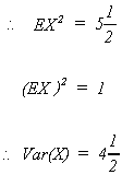
If we wish to find the variance for our winnings we could again use expectations. Namely,

For the coin game
X |
X2 |
P(X) |
X2P(X) |
4 |
16 |
1/4 |
4 |
1 |
1 |
1/2 |
1/2 |
-2 |
4 |
1/4 |
1 |
There are some general rules for mathematical expectation.
RULE 1
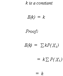
RULE 2
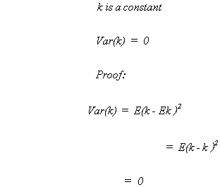
RULE 3
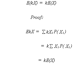
RULE 4
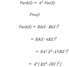
RULE 5
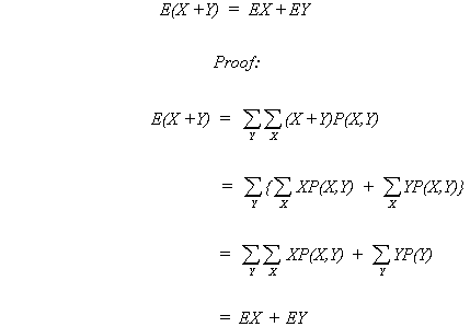
As a note: X, Y are random variables with a joint probability function.
Also,
but,