Classical Economic Time Series Methods
Modeling Dynamic Processes
This part of the lecture notes deals with some classic models using lagged variables. The models discussed are the Koyck Lag, Partial or Stock Adjustment, the Almon Lag, and Adaptive Expectations. The definitive works on these classic models are P. Dhrymes, Distributed Lags, North-Holland, 1981 and H.S. Houthakker and L.D. Taylor, Consumer Demand in the U.S. Analyses and Projections, Harvard University Press, 1970. Other sections of the lecture notes deal with more contemporary issues in time series analysis. Good treatises for the material in the other parts of the lecture notes include T.C. Mills, Time Series Techniques for Economists, Cambridge University Press, 1990 and J.D. Hamilton, Time Series Analysis, Princeton University Press, 1994.

Part 1. Classic Models of Lagged Variables

Suppose, as a simplification of Koyck(1954), that investment in rail cars in the current year, y_t, depends on freight carried in previous years, x_t-j. Without knowing how long it takes the prior freight effects to die out we might specify the model as
1

For sufficiently small d we could neglect the more distant lags. Nonetheless, there remain two problems with the model. First, given the nature of economic data, a variable and its lags are inherently collinear. Second, there is an identification problem even if we were able to overcome the collinearity problem. Namely, the coefficient on x_t provides an estimate of b, as will the pair of coefficients on the once lagged and twice lagged values of x. Both of these problems can be overcome by applying the Koyck transformation.
Whatever is true about the relationship between the current value of y and the history of x must also be true for the previous period observation on y. Hence, we have the pair of relations

2

Multiply the second relation by d
3

Now subtract the result from the original specification of the model and rearrange terms to get

We have solved the problems of overidentification and multicollinearity. However, potentially we have introduced a problem with the error term.
If the error term had the desirable properties of the classical regression model in the original specification, then after the Koyck transformation it no longer possesses them. In fact, the error term becomes a first order moving average, requiring an estimator other than OLS. But the complication doesn't end here. Notice that one of the right hand side variables is y_t-1 and a part of the error term is u_t-1. The model now violates the assumption that the independent variables are statistically independent of the error term. The estimator that immediately suggests itself is the instrumental variables estimator with the correction for the moving average error term. Can you derive the error covariance matrix? One would proceed along the same lines as the procedure used in deriving the error covariance matrix in the autocorrelation case.
Note that the Koyck transformation gives us a model which is a first order linear difference equation. You can use the usual algebra to reach conclusions about the magnitude and sign of d necessary for different patterns of decay in y after a change in x. These impacts of a change in x are worth a further look, neglecting any problems in the error term.
The immediate impact of a one period - one unit change in x is b. One period later y is only bd above its original level. Two periods later y is only bd² above its previous level. With the passage of time the one unit - one time impact on y of a change in x dies out. The impacts can be summarized in the second column of the following table. If the change in x is permanent then the individual period impacts must be summed to find the long run change in y. These sums are provided in the third column of the table.
Impact of a one unit change in x
Period Impact Cumulative
1 b b
2 bd b(1+d)
3 bd² b(1+d+d²)
. . .
. . .
. . .
t bd^t b(1+d+...+d^t)
. . .
. . .
. . .
¥ bd^¥ b(1+Sdⁱ)
The final column is a convergent infinite series provided -1 < d < 1. Using a few lessons from calculus one could show that the cumulative effect is. A way to arrive at the same result and which has a bit of economic content is to consider the long run. Suppose that x has remained fixed for 'a long time'. In this case y also remains unchanged. Making use of this we can rewrite the Koyck transformation as

Hence the long run impact on y of a change in x is the slope coefficient in this model.
Two other useful summary numbers are the mean lag and the median lag. The mean lag is; a lag weighted average of time. The median lag is the length of time necessary for the adjustment to a change in the level of x to be 50% completed. It is computed from.
While the initial Koyck specification was somewhat ad hoc there are in fact two very important economic models which lead to the Koyck model. These are the adaptive expectations model and the partial or stock adjustment model.
Partial or Stock Adjustment
Suppose y_t is income and Q_t^* is desired consumption in period t. The relation between them is. However, it is only in the fantasy world of neoclassical microeconomics that adjustments to desired levels are made in a single period. Instead, the gap between the what was consumed last period and what we desire to consume this period is only partially closed. The result is that the observed changes in consumption are given bywhere gamma measures the speed of adjustment. Notice that the model is backward looking in the adjustment process. Substitute desired consumption into the adjustment equation to get

By successively lagging this last expression for Q_t and substituting back, one can eventually derive the Koyck model which was our starting point in this section.
Adaptive Expectations
Suppose that you plan your purchases of a commodity in this period on the basis of what you expect the price to be next period. Already there is a difference from the stock adjustment model in that you are forward looking. The purchase decision could be modeled as
12

How do you form your expectations for the price in the next period? One possibility is that you revise your expectations for the future on the basis of the error that you have made in the past. That is,

Solve this process for the formation of expectations for x^e_t+1 and substitute into the original relation

Now let us write the original equation for the prior period and multiply it by 1-l.
15

Now subtract (15) from (12) to eliminate the unobservable expectations variable

which can be seen to be the same as the estimating equation in the partial adjustment model. One can also see that by recursive substitution it is possible to work backwards to the geometric lag model we started with earlier.
Cagan (1956) was one of the early users of the adaptive expectations model, but Friedman won the Nobel prize for it. Without going into the details, Friedman's implementation of the permanent income model allowed economists to reconcile the conflict between estimates of the MPC from cross section and time series studies.

Finite Lags
In the preceding we assumed that lag on the independent variable was infinite and that the weights declined geometrically. On the one hand this has freed us of making a determination of the correct lag length. On the other hand it confines us to a very particular shape for the lag weights and presents some difficulty in estimation. If the number of lags are known to be finite, or reasonably approximated by a finite number, but the lag weights may not lie along a nice smooth geometric line then we may want to consider the Almon Lag as an alternative. The Almon technique allows us to choose the length of the lag structure, its shape, and its smoothness while economizing on the number of parameters to be estimated. That we can use a polynomial of sufficiently high order to approximate any function is a well known result and forms the basis of the technique.
Suppose we have the following model
17

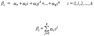
If we allow the coefficients, b₁ ... b_k, to lie along an integer polynomial of degree q of the sort

Then we need to estimate an intercept and q slope coefficients instead of the intercept and k slopes in the original specification. Let

Substituting into the model in (17)

Applying least squares

Example
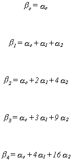
Suppose we believe the polynomial to be quadratic, q = 2, and the number of lags to include the current, once lagged, twice lagged, and thrice lagged values of the explanatory variable, k=4.
22

Then

<

We need estimate only three coefficients instead of the five in the original specification. Furthermore, the estimation doesn't really involve any transformation of the right hand side variables. Instead we can use restricted least squares. Note that

So we could estimate y = xb + u subject to the restrictions

Through suitable use of the F statistic one could test for the appropriate degree of polynomial and lag length.

The Long Run and the Short Run
This classical approach to the characterization of long run and short run results is presented here because it is associated with modeling dynamic processes. In the chapter on modern time series we will again address the long run and the short run in the discussion of unit roots, cointegration and error correction mechanisms.
For the time being we suppose that we have the following very simple consumption function

q is the rate of consumption of some commodity. This is a flow.
y is income. This is a flow.
S is the stock of commodity q accumulated up until time t. This is a stock. This may be thought of in both the psychological and physical sense. In the former it is an indicator of habit formation.
If< 0 then we interpret S as a physical stock.
If> 0 then we may interpret S as a psychological stock. The commodity represented by q is habit forming.
The rate of change of the stock of the commodity with respect to time is given by

where d is the depreciation rate on S. In the steady state S is a constant over time so the consumption path is described by

Plugging back into the original commodity demand function gives us

Collecting on the steady state consumption of the commodity

Since this is the steady state the coefficient on y_t may be termed the long run income effect. By definition d < 0.
Durable Goods
If< 0 thenand clearlyin the steady state. In the long run the income effect is smaller than the short run income effect. A rise in income gives a sudden burst to the income effect, but in the long run it becomes dampened.
Habit Forming Goods
If> 0 butthenand. The conclusion is that the long run income effect is larger than the short run income effect.
Economic theory suggests that for durable goods h^{short run} > h^{long run} and for habit forming goods h^{short run} < h^{long run}. The evidence is that
AUTOS
h^{short run} = 5.46 from time series
h^{long run} = 1.07 from cross section
BOOZE
h^{short run} = .29 from time series
h^{long run} = .69 from cross section
We conclude that time series results are short run elasticities and that cross section results are long run elasticities.