DATA PROBLEMS: Missing Data
By way of introducing the area of concern and organizing our thinking, consider the
following table. The first row describes how it might come to pass that some of the data
is missing in both cross section and time series data. If the data is missing for a reason
that has nothing to do with the behavioral content of the model then the only consequence
is that our estimators are less efficient. This is solely a result of sample size. In a
cross section one could not predict which observations will be missing on the basis of
some knowledge about the respondent pool, for example.
There is a class of problem in which observations are missing as a result of the process
being modeled. This is the third row of the table. For example, we might be modeling the
purchase of refrigerators. If the purchase price of a refrigerator is never below $200,
then in our sample we will never see a household that would have liked to purchase a
refrigerator for $175.
|
Cross Section
|
Time Series
|
Nature of Problem
|
Respondent fails to answer question
|
Model needs monthly, we have quarterly
|
Missing data unrelated to complete observations
|
Lowers efficiency
|
Lowers efficiency
|
Gaps in data systematically related to behavior to be modeled
|
See any text on censored and/or truncated data. The classic
estimator for this genre is Tobit.
|
In the next table we categorize the missing data problems we can deal with at this
point. Basically, you can be missing data for either the dependent variable or for some of
the independent variables. The problem, or question, is how to leverage the data that one
does have in order to increase the efficiency of the estimator.
|
ya, xa
|
na complete observations
|
Case 1
|
___, xb
|
nb missing observations on yb
|
Case 2
|
yc, ___
|
nc missing observations on xc
|
CASE 1 Missing observations for
dependent variable
Let be a predictor for yb so the least
squares estimator for the coefficient vector in this filled data set is
 . In general we can write the normal equations as x'y = x'x, so make
this substitution for the data-on-hand estimator, ba, and the missing-data
estimator, bb:
 .
.
Define F = [xa'xa + xb'xb]-1xa'xa
so I - F = I - [xa'xa + xb'xb]-1xa'xa,
or I-F = [xa'xa + xb'xb]-1xb'xb
since I = [xa'xa + xb'xb]-1[xa'xa
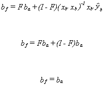
+ xb'xb]. Then the filled data estimator is bf = Fba
+ (I-F)bb, with Ebf = Fb + (I-F)Ebb.
Unbiasedness is seen to depend on Ebb.
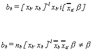
Method 1
Let i be a column vector of ones. For the missing data estimator we will replace each
missing observation on y by the mean of the observations on ya. Then where
where and
and is a row
vector of variable means. Note
 where
where is a
column vector of variable means. Making the obvious substitution we get
Method 2
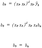
Get ba = (xa'xa)-1xa'ya
then build b = xbba and
Also,
Now for the variance. We have
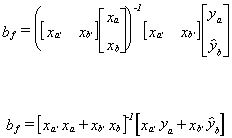
Substitute in for 

factor out xa'ya and substitute in for ya
Post-multiplying bf by its transpose and taking expectations will give us
the variance of our pooled estimator.

If you multiply xa'xa through to the right then the last pair of
square brackets cancel. Now factor (xa'xa)-1 out of the
remaining terms and one is left with . There is no gain in
efficiency from using the filled estimator. In practice, because one must estimate s2, it will appear that the estimated standard errors of
the filled estimator are smaller. Do you see why this is so? It depends only on the number
of observations the computer uses in the calculated estimate of s2.
EXAMPLE: Left Hand Side Missing Data
Suppose that the entire correct data set is shown in the following table.
| Y |
x |
| 0 |
0 |
| 2 |
1 |
| 1 |
2 |
| 3 |
1 |
| 1 |
0 |
| 3 |
3 |
| 4 |
4 |
| 2 |
2 |
| 1 |
2 |
| 2 |
1 |
If we use all of the observations to estimate a simple linear model then the result, with
t-statistics in parentheses, is
| y = |
.8333 |
+.666x |
+e |
n=10 |
|
(1.75) |
(2.81) |
|
|
But suppose that for some reason we do not observe the last four data
points for y. Using the abbreviated data set our regression result is
| y = |
.6476 |
+ .6341x |
+e |
n=6 |
|
(1.43) |
(1.55) |
|
|
Using the coefficient estimates from this abbreviated database we
construct fitted values for the last four observations on y, bringing our total number of
observations back up to ten. Running the regression with 6 observed values for y and 4
fitted values for y gives us the following result
| y = |
.9268 |
+.6341x |
+e |
n=10 |
|
(2.32) |
(3.179) |
|
|
Notice how much higher the t-statistics are than those in the regression
when we had all of the correct data. This is contrary to the derived result. We had
asserted above that our filled estimator was no more efficient. This is another case of
the computer not really knowing what is going on. It must compute an estimate of the error
variance from the observed data for use in an estimate of the variance of the coefficient
estimator. In our filled data set the last four observations contribute nothing to the sum
of squared errors, but the denominator is still 10. The consequence is that the estimate
of the error variance is understated. The implication is that the careless researcher will
use this filled estimator, which is no more efficient than the estimator based on the
abbreviated data set, not question the very high observed t-statistics and reject too many
null hypotheses.
Case 2 Missing observations on
the right hand side.
Simple Regression
We have the simple regression model ya = a + bxa + ua and the additional nc
observations on yc, but the observations on xc are missing. One
possibility is to use to fill the blanks. This won't work since
these terms would get zero weight in
 . We would gain nothing for
our effort.
Another possibility is to use the reverse regression  to construct
 then build a set of fitted values for xc according to
  . Now apply OLS to the filled model
  . The
sampling distribution of the OLS estimator for the parameter vector is unknown in this
scheme so we can say nothing about unbiasedness and efficiency.
EXAMPLE: Missing data on the right hand side
For this example we use the same data as in the previous example. If we run the simple
regression with y on the right hand side, x on the left hand side and using only the first
six observations then we get the following result
| x = |
.7633 |
+.3817y |
+e |
n=6 |
|
(.24) |
(1.55) |
|
|
Using these results to fill in for the missing values for x and applying OLS we get
| y = |
.7670 |
+ .8685x |
+e |
n=10 |
|
(1.59) |
(2.90) |
|
|
Notice that the slope estimate is higher than when we have all the data, as it was in
the prior example. This is coincidence. It depends on the realization of the data which is
available to us. That is, it is sample specific. Also, the t-statistic on the slope
estimate is higher. This is not coincidence, for the same reason given in the earlier
example.
Multiple Regression
Given the available data we have the following model
 (1)
(1)
for which we have na observations. We have another nc observations on yc and zc.
From the additional observations we might fill in for the missing xc. We could use the first na observations on x and z in the following equation
 (2)
(2)
In the last nc observations we would then substitute
in for x

The model then consists of the equations (1), (2), and (3). To operationalize
let  .
.
Now  . This method allows us to use more information about the
dependent variable and z in our estimation of
  . This should
provide us with a more efficient estimator.
EXAMPLE: Right Hand Side Missing Data: Multiple
Regression
We are given the following aggregate data for Taiwan. One could estimate a production
function using this data
YEAR
|
CAPITAL |
LABOR |
OUTPUT |
| 1958 |
17804. |
275.50 |
16608. |
| 1959 |
18097. |
274.40 |
17511. |
| 1960 |
18272. |
269.70 |
20171. |
| 1961 |
19167. |
267.00 |
20933. |
| 1962 |
19648. |
267.80 |
20406. |
| 1963 |
20804. |
275.00 |
20832. |
| 1964 |
22077. |
283.00 |
24806. |
| 1965 |
23445. |
300.70 |
26466. |
| 1966 |
24939. |
307.50 |
27403. |
| 1967 |
26714. |
303.70 |
28629. |
| 1968 |
29958. |
304.70 |
29905. |
| 1969 |
31586. |
298.60 |
27508. |
| 1970 |
33475. |
295.50 |
29036. |
| 1971 |
34822. |
299.00. |
29282. |
| 1972 |
41794. |
288.10 |
31536. |
Using all of the data one obtains
| Q = |
-1.6900 |
+ 2.454L |
+ .4326K |
+ e |
|
(-2.97) |
(4.06) |
(5.48) |
|
But suppose the last three observations on capital are missing. Using just the first
twelve data points we observe
| Q = |
- 1.763 |
+2.1193 L |
+.5406 K |
+ e |
|
(-1.76) |
(2.06) |
(2.39) |
|
If we use the first 12 observations on capital and labor to estimate a linear regression
the result is
| K = |
-2.926 |
+ 3.8273 K |
+ e |
|
(-3.35) |
(4.95) |
|
The R2 is .71 and both coefficients are significant; L does quite a good job
explaining capital. Use these coefficients to construct a fitted series for capital so
that we have a total of 15 observations and run the original model again.
| Q = |
- 1.7610 |
+ 2.4428 L |
+ 5.406 K |
+ e |
|
(-1.40) |
(1.58) |
(1.57) |
|
The coefficient on labor does not change a great deal. Compared to the complete correct
data set, the coefficient on K has changed by 25%, this is a big change. Compared to
either the full or abbreviated data set the estimated coefficient standard errors have
apparently gotten larger, the t-statistics have fallen.
 . In general we can write the normal equations as x'y = x'x, so make
this substitution for the data-on-hand estimator, ba, and the missing-data
estimator, bb:
 .
. 


 . The
sampling distribution of the OLS estimator for the parameter vector is unknown in this
scheme so we can say nothing about unbiasedness and efficiency.
 . This method allows us to use more information about the
dependent variable and z in our estimation of