4. Seemingly Unrelated Regression
4.1 The Problem
There may be several equations which appear to be unrelated. However, they may be related by the fact that
1. some coefficients are the same
2. the disturbances are correlated across equations
3. a subset of right hand side variables are the same, although all observations are not the same.

The estimator proposed here was developed by Zellner. The classic example uses Grunfeld's investment data. This estimator was the basis for the development of three stage least squares.

4.2 Set Up

We suppose that the i^th equation in a set of n equations is given by

where Y_i is Tx1, X_i is Txk, b_i is kx1, and U_i is Tx1. The whole set of n equations can be written as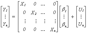

or more compactly as The error variance-covariance matrix is

(4.1)

Each diagonal term is a TxT variance-covariance matrix for the disturbance of the i^th equation. The off-diagonal TxT blocks are contemporaneous and lagged covariances between errors of pairs of equations. We assume the following
(4.2)
For any given equation the disturbance is homoscedastic and non-autocorrelated. For i¹j we have non-zero correlation between contemporaneous terms of the two equations, but zero correlation between lagged disturbances. Substituting 4.2 into 4.1 we have 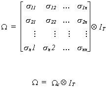Note that W is of full rank.

Caveats

1. If the between equation covariances are zero then there is no advantage to applying Zellner's SUR. It is equivalent to OLS. However, larger covariances mean that there is a larger efficiency gain in using SUR.
2. If the same data is used in each equation, the actual numbers are the same, then there is no advantage to applying Zellner's SUR. It is equivalent to OLS. The more dissimilar the Xs, the greater the gain in using SUR.

Estimation

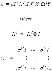
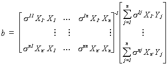
When W is known we can construct the BLUE estimator

The BLU estimator may be written as

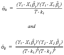
As a practical matter we often don't know W and must estimate it. A proposed two step procedure is as follows: 1.a. Fit the n equations separately to obtain the residual vectors

1.b. Estimate the variances and covariances as

1.c. Use the to obtain S^-1 as an estimate of W^-1.

2. Construct The proof from the random effects - error components chapter can be adapted to show when b^* is unbiased.

NOTES

1. One could use a likelihood ratio statistic to test for non-zero covariances between equations. The test statistic is

where S_n² is the estimate of the error variance when applying least squares to each equation individually and W is the estimate of the error covariance matrix when there are contemporaneous cross equation covariances. The number of degrees of freedom for this c² is n(n-1)/2.

2. Occasionally you will see the Zellner estimator iterated. That is, estimate the slopes by OLS, construct an estimate of the error covariance matrix, reestimate the slopes, reestimate the error covariance matrix, and so on. The iterated estimator can be shown to be the maximum likelihood estimator. However, the estimator outlined above is the feasible generalized least squares estimator. Therefore there is no gain from applying the iterations. In large samples the ML and FGLS estimators have the same properties.

An Example

Investment = f₁(expected profits)

expected P = f₂(value of outstanding stock at end of year)

F_t = market value at end of year

C_t^* = desired capital stock where C_t^* = b_o + b₁ F_t

C_t = existing capital stock

By substitution we see that desired net investment is C_t^* - C_t = b_o + b₁ F_t - C_t

Let the fraction of desired net investment that is actually realized be denoted by q₁. Then realized net investment is

Depreciation investment is q₂C_t so

We have data on Westinghouse and G.E. for the period 1935-1954. Estimating the parameters for the two companies separately

G.E.: I_t = -10.0 + .027 F_t-1 + .152 C_t-1 Rbar² = .671

(.016) (.026)

West: I_t = -.5 + .053 F_t-1 + .092 C_t-1 Rbar² = .714

(.016) (.056)

The numbers in parentheses are standard deviations of the coefficients. The estimated error covariances are

Our test statistic for non-zero covariances, with one degree of freedom is

l_LR = 20 ( ln(660.22)+ln(88.67) - ln(660.22 x 88.67 - 176.4²))

l_LR = 15.16

This is a good deal larger than the critical value for any reasonable level of significance so we reject the null hypothesis of diagonal covariance matrix. If we use the fact that the contemporaneous covariances are not zero then the results change slightly to

G.E.: I_t = -27.7 + .038 F_t-1 + .139 C_t-1

(27.00) (.013) (.023)

West: I_t = -1.3 + .058 F_t-1 + .064 C_t-1

(7.0) (.013) (.049)

The standard errors of the coefficient estimators have narrowed some. It is also possible to see the efficiency gain in two dimensions.