|
|
||
|
|
||
V. HYPOTHESIS TESTING
As already acknowledged we know little about the values of population parameters that define the probability distributions of the world. In the previous section it was our goal to estimate these parameters. Often we may have some prior notion of what these parameters might be. Consequently, we may wish to test our hypotheses. Our prior guess is called the null hypothesis and is denoted H0, it is most often what we believe to be true. On the basis of observed sample information we decide to either accept or reject the null hypothesis.
In making our decision to reject or accept the null hypothesis we must consider
the costs that will accrue from making an incorrect decision.
What is an incorrect decision?
1. Rejecting a true null.
2. Accepting a false null.
Example: Consider a court case. The defendant is being tried for a violent crime. There are two possible states of the world: He committed the crime or he did not. The jury can return one of two verdicts: guilty or not guilty.
Let us tabulate the problem:
|
|
||
|
|
||
H0: innocent
H1: guilty
Two errors:
1. Type I, reject true null,![]()
convict an innocent man
2. Type II, accept false null,![]()
free a convict
In the American justice system the belief is that sending an innocent person to
jail is the more serious error, so we specify that to be the null hypothesis. The system
is further designed to make the probability of a type I error as small as possible. All
other things equal, however, this results in driving up the probability of a type II
error.
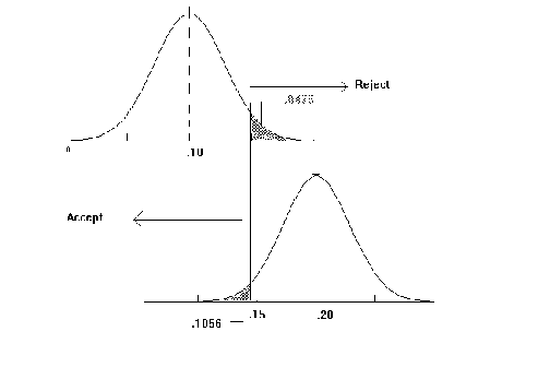
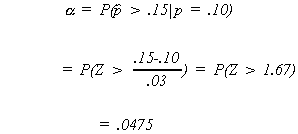
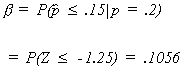
Example: Vita Synthetics has just developed a dietary supplement. It is purported to reduce cholesterol in arteries. The FDA will not allow us to market the drug without strong evidence that it will work on humans. They decide to test our hypothesis and select 100 males. From past experience the FDA knows that in about 10% of all males cholesterol declines naturally. They have decided that there must be sufficient evidence to decide that the drug reduces cholesterol in 20% of all middle age males.
H0: P = .10
H1: P = .20
The null hypothesis is that the new drug does noting to affect cholesterol levels, even though we may hope that this is not the case.
Arbitrarily the FDA establishes the following decision rule
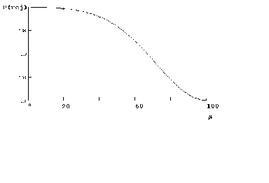
We know ![]()
Therefore, there is a probability distribution for each hypothesis. The diagram shows the region for observed proportions which would lead us to reject the null when it is true; the top panel. It also shows us the region of observed proportions for which we would accept a false null.
We need an estimate of the variance of the sample proportion in order to construct
our test statistic.
![]() UNDER NULL
UNDER NULL
TYPE I ERROR
![]() under the alternate
under the alternate
TYPE II ERROR
The preceding was an example of a simple hypothesis test because there was only one alternative to the null hypothesis. A richer class of hypothesis tests would be those that include a range of alternatives.
Example: A manufacturer claims that his machinery puts 100 paper clips in every box, on average. We doubt his claim. Believing that he puts in fewer. It is known that the population standard deviation is 5.
![]()
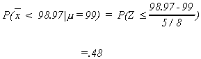
We take a sample of 64 boxes and find![]() .
.
With![]() do we have a case against the
manufacturer.
do we have a case against the
manufacturer.
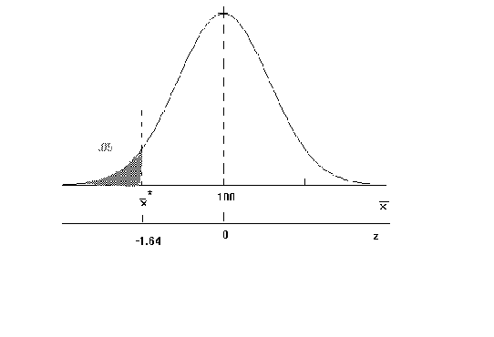
The critical Z is -1.64
since![]() we reject the null hypothesis.
we reject the null hypothesis.
The above was a one tail test. We could do a two tail test.
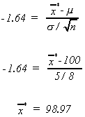
Example: (student t)
The weight of bananas in a box car is known to be![]() . But the parameters are unknown to us. Our South American supplier
claims that on average a box car of bananas weighs 50,000 lbs. Since underweight box cars
are costly to us and over weight cars are known to have a lot of tarantulas in them we
wish to test his claim.
. But the parameters are unknown to us. Our South American supplier
claims that on average a box car of bananas weighs 50,000 lbs. Since underweight box cars
are costly to us and over weight cars are known to have a lot of tarantulas in them we
wish to test his claim.
![]()
Because we don't wish to irritate a sympathetic government we choose![]()
We randomly weigh nine box cars and observe
![]()
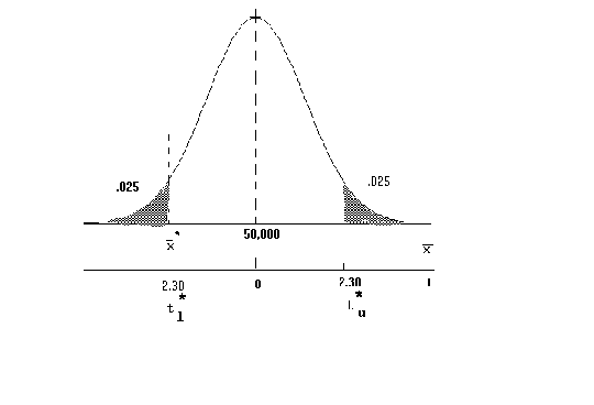
The upper and lower critical values are found from
and 
since![]() we accept the claim of our
South American client.
we accept the claim of our
South American client.
POWER OF A TEST
Recall that in our first example of hypothesis testing we considered the null and alternate
![]()
and were able to calculate a single value for![]() , the probability of a type II error. When rejecting the null, we do so in
favor of a specific alternative.
, the probability of a type II error. When rejecting the null, we do so in
favor of a specific alternative.
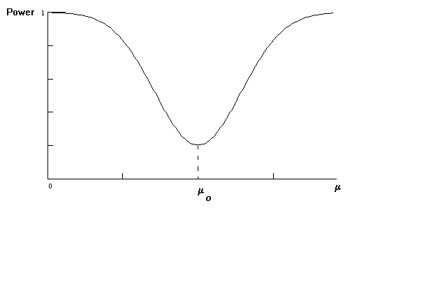
However, in the second example we considered
![]()
As a consequence, the null is incorrect for any![]() and so there must be a multitude of type II errors,
and so there must be a multitude of type II errors,![]() . Now one would / could reject the null in favor of an infinity of
alternatives. In a sense this is problematic since for sufficient data we can reject any
null in favor of this infinity of alternatives.
. Now one would / could reject the null in favor of an infinity of
alternatives. In a sense this is problematic since for sufficient data we can reject any
null in favor of this infinity of alternatives.
Let us define
Power = P(REJ H0)
and since ![]() = P(accept a false H0)
= P(accept a false H0)
Power = 1 -![]()
Power measures our ability to differentiate between the null and the true state of the world. We would hope that as the true state of the would differs increasingly from H0 that P(Reject H0) would increase.
In fact, such is the case for tests on![]() .
.
Let us return to the paper clip example
![]()
and set power on the ordinate and possible values of![]() on the abscissa.
on the abscissa.
Calculating a few points:
1. ![]() which we know is .05
which we know is .05
2. Suppose, unknown to us,![]()
![]()
3. 
For a two tail test the power curve would appear as
TESTS OF HYPOTHESIS AND POPULATION VARIANCE
Two tail test: Recall the weight of bananas in a box car problem. From a sample of 9 cars it is found that
s2 = 8100
Suppose we wish to test
![]()
at the![]() level of significance
level of significance
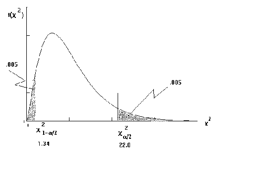
the diagram shows the critical values.
Calculate the observed test statistic
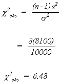
The observed test statistic is in the acceptance region.
A power curve for tests of![]() would be
calculated in the same fashion as tests on
would be
calculated in the same fashion as tests on![]() .
.
A NOTE ON THE DISTRIBUTION OF s2
Recall if![]() , then
, then
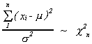
Also
![]()
or
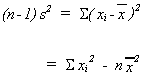
Note that if![]() then
then![]() . Also
. Also![]() .
.
Let us add![]() to
to![]() and take it out again
and take it out again
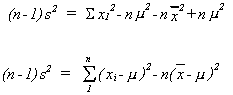
Now divide both sides by![]()
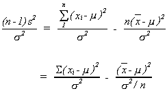
The first term on the right is![]() , the
second is
, the
second is![]()
![]()