SPECIFICATION PROBLEMS: Part 2

Functional Form
Functions Linear in Parameters
Almost every modern econometrics textbook presents material on nonlinear estimation. This seems to me to be much ado about nothing. To begin with, the small sample properties of these estimators are not well understood. At best we can say something asymptotically. With OLS we can say a great deal both in large samples and in small samples.
Secondly, the nonlinear estimation routines are computationally burdensome. They rely on a hill climbing algorithm that either minimizes the sum of squared errors or maximizes the likelihood function. Most software packages offer at least two algorithms for this. In the fine print they always remind the user to choose starting values carefully. There is usually a caveat that choice of functional form is important for avoiding local minima or maxima.
A third problem is that economic data is often very flat. That is, for the observed data, the ascent on the likelihood function may not be very steep. As a result the algorithm may wander around on likelihood function until the number of iterations is used up. The closing round estimates may be quite different depending on the chosen starting values for the model parameters.
The final reason that non-linear estimation is a great deal of noise to little effect is that there are other useful alternatives. Not only are there other alternatives, but in most cases we would be quite justified in using the alternative. We know from the Weierstrasse Theorem that we can approximate, to any desired degree, any continuous and continuously differentiable function with a polynomial of sufficiently high degree.
There are exceptions to these comments. The most notable one is in time series analysis. If ARIMA models are to be estimated by maximum likelihood then nonlinear routines are the only way to go.

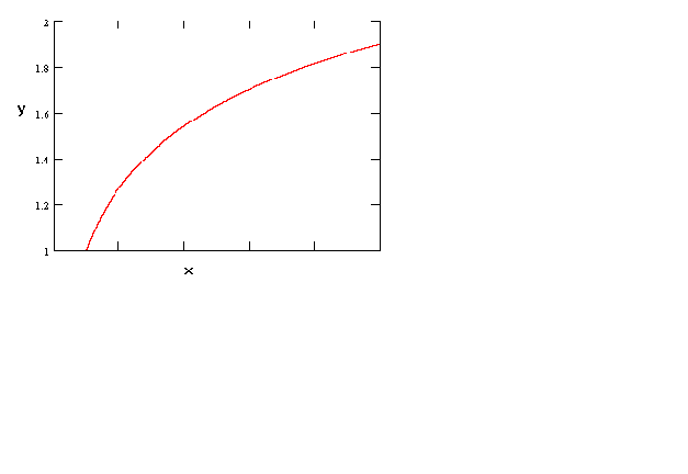
Figure 1

y = a + b ln(x)

As a first example consider the above figure. This is just the semi-log function .

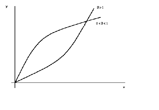
Figure 2

ln(y) = a + b ln(x)
The above example is the log-log function. Whether the curve is concave or convex depends on the size of b. If there were another right hand side variable or two then the function would be the familiar Cobb-Douglas function. By simply changing the sign on b we can get a curve that looks like an indifference curve or an isoquant, as in the following figure. By altering the magnitude of b it is possible, in the context of indifference curves, to show a relatively stronger preference for one good or the other.
Figure 3

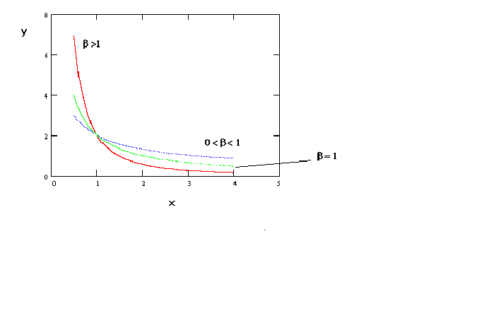
ln(y) = a - b ln(x)
If one uses the inverse of the independent variable then one gets a curve as in figure 4.

Figure 4 y = a + b (1/x)
The curve is convex and approaches an asymptote from above.
This might be useful for estimating a money demand function. Elsewhere in this chapter you will encounter the Box-Cox transformation. This is the usual model for money demand. As you will see, it is an analytically cumbersome technique.

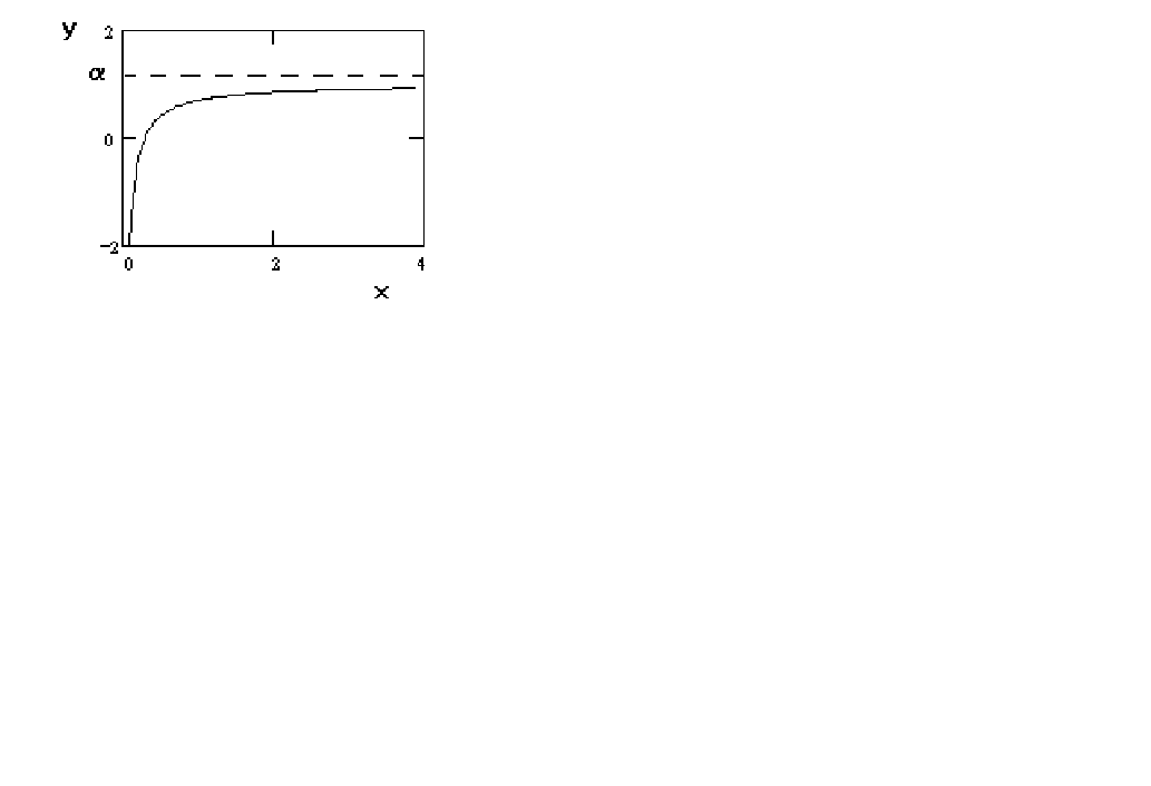
Figure 5    y = a - b (1/x)

In figure 5 we just change the sign on the coefficient in the 'money demand' function. The result is that it is concave and approaches the asymptote from below.
In figure 6 we can produce a sigmoidal shape by proper choice of the parameters. For example, a production function might have this shape if over the relevant range of output there is not a negative marginal product. For most problems in economics this seems quite plausible.

Figure 6     ln(y) = a + b (1/x)

In Figure 7 we have a parabola.

Figure 7     y = a + bx + gx²
By suitable choice of parameters we could flip it over and have an average cost curve.
Finally, although the coefficients have been chosen to exaggerate the shape, a cubic function can be chosen to create a production function or cost function that is well behaved.

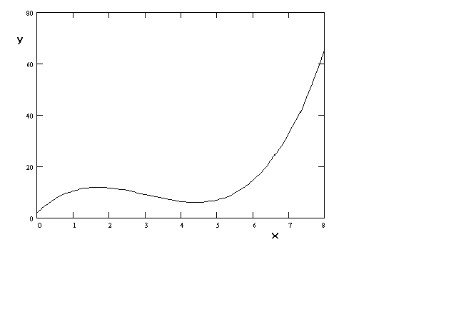
Figure 8 y = a+ bx + gx² + dx³

The curves in figures 7 and 8 do present their own challenges at the time of estimation. It is often found that when the independent variable is entered on the right hand side in polynomial form the problem of multicollinearity rears its ugly head. This can be overcome in part, for example, by estimating an average cost curve instead of a total cost curve. So doing entails dropping, say, the cube term from the function. Another solution is found in the use of orthogonal polynomials. See F.A. Graybill, An Introduction to Linear Statistical Models, McGraw-Hill, 1961, Pp. 172-182.

2. The Box-Cox Transformation
We begin with the observation that if we define f(z) as follows

then for

The last line is found by applying L'Hopital's Rule. Given the flexibility of this transformation it is suggested that the classical linear regression model be written as

The least squares estimates are

(i)

One would proceed by any one of several methods. The easiest would be a Taylor Series expansion of (i). Use the OLS estimates of b as a starting point then conduct a grid search over .

A Table of Functional Forms and Properties can be found here.

An interactive look at functional forms