6.3 Estimation
6.3.1 Single Equation Methods
6.3.1.1 Instrumental Variables
We begin with Instrumental Variables (IV) estimation for several reasons. First, it is easy to show that the estimator is consistent. Second, as we shall see, it is easy to show that our other systems estimators are equivalent to the IV estimator. Third, the IV estimator has a number of applications outside of systems models, making it rather more general in applications.
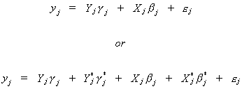
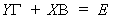
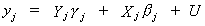
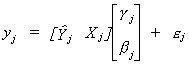
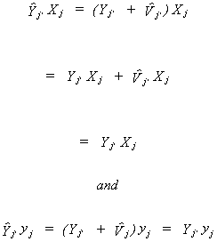
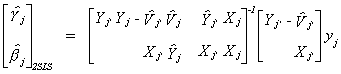
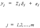
Suppose that the j^th equation is

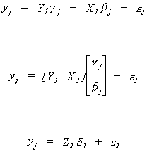
In an earlier section we showed that d_j cannot be consistently estimated because some of the variables on the RHS are correlated with the error term. To get around this predicament we define W_j: Tx(m_j+k_j) to satisfy

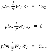
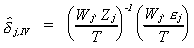
The IV estimator is

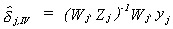
substituting for y_j we get

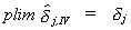
Applying Slutsky's Theorem we can see

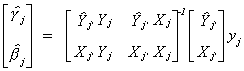
The asymptotic variance of the IV estimator (the variance of the asymptotic distribution) is

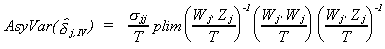
with

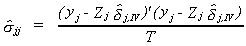
a consistent estimator.
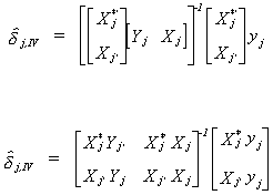
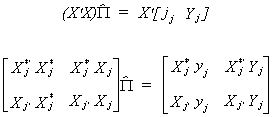
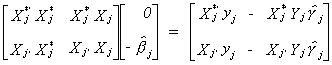
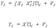
Suppose that the system is exactly identified. Then

The * designates excluded variables. The number of excluded exogenous variables, k_j^*, is equal to the number of included endogenous variables, m_j. Let the matrix of instruments be made from the included and excluded exogenous variables, W = [ X_j^* X_j ].
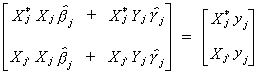
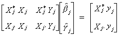
so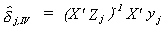. Or, expanding the matrices

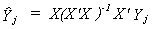
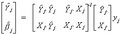
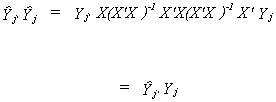
We can show the equivalence of the IV estimator and the Indirect Least Squares estimator. Begin by going back and estimating the reduced forms coefficients for the edogenous variables in the jth equation.

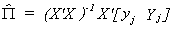
Premultiply by (X'X)
12 (a)

From our work on identification we know that the following restrictions must hold

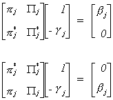
Now rewrite (a) as

Postmultiply the above result by to get

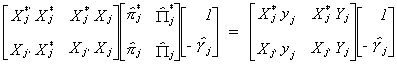
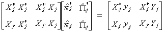
The product of the second and third matrices on the left hand side of the equation we recognize as . Making this substitution yields

Doing the multiplication and rearranging terms gives the following

Now factor out the estimated parameter vector
20 (i)

We can see that (a) and (i) are the same thing !
When the equation is overidentified ILS and IV are not equivalent. ILS produces more than one estimate of the overidentified parameters, while IV uses the overidentifying restrictions in producing its one estimate of each parameter.
What Does IV Do?
The following three figures help us understand what IV does. The first figure shows the normal case of the classical regression model in which no RHS variable is correlated with the error term. The second figure illustrates what happens when the zero correlation assumption is violated but we apply OLS anyway. The third figure shows the IV correction.

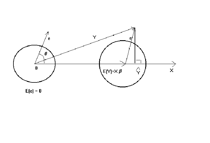
Figure 1: The Classical Regression Model

In the above figure Y is the dependent variable, X is the set of k independent variables. The circles represent a contour of the normal distribution in the space in which the dependent variable lies. The idea behind the contour is similar to the use of indifference curves in micro theory. All the points on a contour are equally likely to occur. Points on a smaller circle are more likely to occur; that is, they are higher on the probability density function. e is a particular realization of the error term. The particular realization of the error term is added to E(Y) to give the realized value of the dependent variable. OLS then projects the realized dependent variable onto the space spanned by the columns of X. Since the mean of the error term is zero, we are adding zero on average to E(Y). On average then our OLS projection would give us E(Y) = Xb.

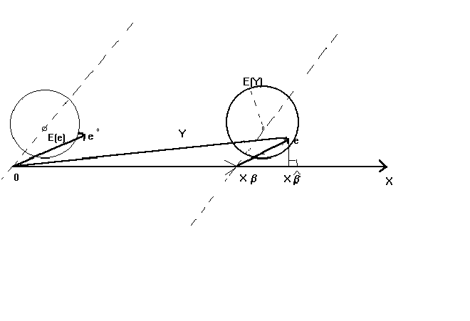
Figure 2: OLS When E(X'U)¹0

The principle difference between the first and second figures is that the mean of the error term, conditional on X, is not zero. We have drawn it so that there is a positive correlation between X and the error term. That is, the center of the error term contours is no longer at the origin, nor is it the axis on which it lies at right angles to the space spanned by X. Thus we are always adding a positive term to Xb. The E(Y) is now located to the northeast of Xb. We will, on average, be dropping a perpendicular from E(Y) onto the space spanned by X. As you can see from the diagram we will overshoot Xb by some amount, even on average. Our conclusion is that OLS produces biased estimates of the model parameters. Increasing the sample size won't correct things since all we accomplish is to make the contours tighter. Hence, OLS is also not consistent.

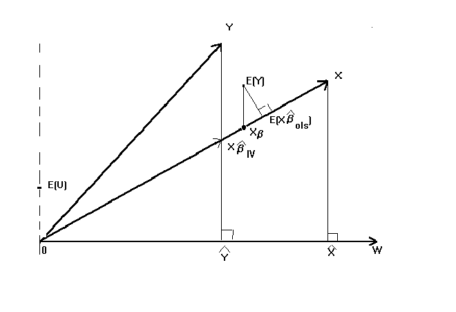
Figure 3: The Instrumental Variables Projection

In figure 3 the error contours have been suppressed to make the figure easier to follow. The realization of the dependent variable, Y, is shown. As is the space spanned by the 'independent' variables, X. The non-zero error term, correlated with the RHS variables, is shown as before. The figure shows that E(Y) when projected orthogonally onto the space spanned by the RHS variables couses us to overestimate Xb. Added to the picture is the space spanned by the set of instruments.
IV first projects the RHS variables onto the space spanned by the instruments, W. Then the dependent variable is projected onto this set of fitted values. As you can see from the picture, when the dependent variable is projected onto W it results in an oblique projection onto the original set of RHS variables. The result is that, at least in large samples, we will correctly estimate Xb with greater likelihood.
The algebra is straightforward. We do the general case in which an equation is overidientified because it provides a lead-in to the next section. We suppress the subscript for the equation number.
Recall that Z is the full set of RHS variables, y is the dependent variable, and W is the set of instruments. In the first step project the RHS variables onto the set of instruments

Replace the original RHS variables by their fitted values and estimate the original set of parameters

From the last line we can see that in IV we are really using a set of fitted values of the dependent variable that have been created by projecting the dependent variable onto the space spanned by the instrumental variables.

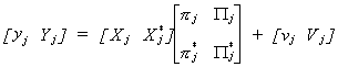
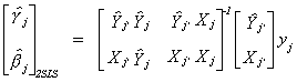
6.3.1.2 Two Stage Least Squares
We have the structural model
23 (i)

which can be written in reduced form as
24 (ii)

Our problem is that the system is overidentified. The consequence is that we cannot use either ILS or the simple IV estimator outlined in the sections preceding the earlier discussion of what IV does. We need to devise a method that uses all of the information in the exogenous variables.
We will consider the j^th equation of (i)
25 (iii)

The usual problem is that Y_j is correlated with the error. IV solves this problem by choosing as instruments a set of variables which are correlated with Y_j, but not with the error term. What we plan to do is use linear combinations of all the exogenous variables in place of the endogenous variables which are included on the RHS of the equation. To construct the linear combinations of the set of all exogenous variables we run the regression

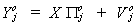
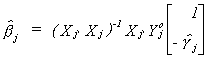
The fitted values of the included endogenous variables are given by

Note that (X'X)^-1X'Y_j is part of the matrix of reduced form coefficients. With this result we can rewrite the model in (iii) as 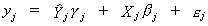. After factoring out the coefficients we can write this in matrix form as

Now apply least squares

Now X(X'X)^-1X' is idempotent so

Since the exogenous variables are independent of the error term and the fitted endogenous variables are orthogonal to the residual we can also write

Making these substitutions, the Two Stage Least Squares estimator is

Suppose the model is exactly identified so that k_j^* = m_j. In this case X_j^* would work equally well as the set of instruments as . If you go back to equation (i) on page 21 and make this substitution you will see that ILS, IV and 2SLS are all the same in the exactly identified case.
Finally, since the IV estimator is known to be consistent, we also know 2SLS to be consistent.
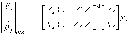
6.3.1.3 Limited Information Maximum Likelihood
We are interested in the j^th structural equation once again. We begin by looking at a partitioning of the reduced form that corresponds to the j^th structural equation

To economize on notation a little bit we will write this as

The error covariance matrix is written as

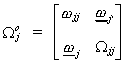
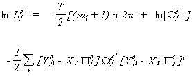
The log of the likelihood function for the joint density is

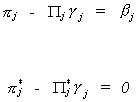
The idea is that we will maximize the likelihood for the equation of interest subject to the constraints that we developed in the section on identification. Namely,

In the exactly identified case we can maximize the likelihood then go to the constraints to solve for the structural coefficients. We conclude also that LIML is, therefore, equivalent to ILS, IV, and 2SLS in the exactly identified case. Also observe that the likelihood function is equivalent to that for the SUR model.
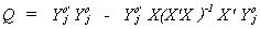
Returning to the over identified case, construct the concentrated likelihood function. First, find

Solve for and substitute back into the log likelihood, this will give us the likelihood in terms of only the reduced form coefficients.

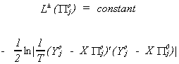
Now form the lagrangean

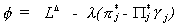
and determine

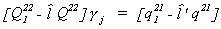
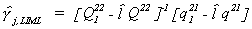
THEOREM
The LIML estimates for b_j andare respectively
a) endogenous coefficients

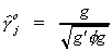
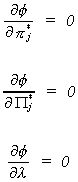
where the normalization rule is and g is the solution to 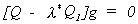. In order for there to be a solution the part in brackets must be singular. Therefore, l^* is found as the maximum root of the determinantal equation 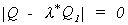. So we conclude that g is the characteristic vector corresponding to l^*. Note that the root can be solved from .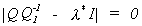

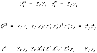
Q is an m_j+1 x m_j+1 matrix of RSS in the regression of all the endogenous variables of equation j on all of the exogenous variables of the system.

Q₁ is an m_j+1 x m_j+1 matrix of RSS in the regression of all the endogenous variables of equation j on only those exogenous variables included in the j^th equation.
b) exogenous coefficients

LEMMA
(i)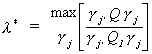
(ii) l^* £ 1

Proof:
(i) Recall from linear algebra

where l₁ is the largest root of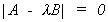
(ii) We can write Q₁ = Q + D where D is a positive semi definite matrix. So

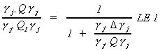
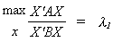
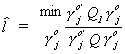
The Lemma leads us to a minimum variance ratio interpretation of the LIML. Consider the j^th structural equation in its original form and a version which includes the entire set of exogenous variables

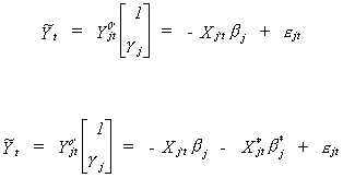
Incidentally, comparing these two specifications of the j^th equation could form the basis of a test for the exclusion restrictions of the structural model.
Define two sets of residual sums of squares corresponding to the two specifications of the j^th structural equation.

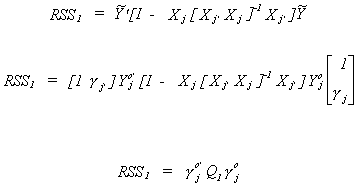
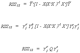
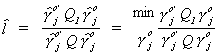
Now construct the ratio

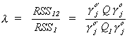
The trick is to pick the coefficients on the endogenous variables, , so that l is maximized. Or, 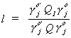is minimized. Call this a minimum variance ratio estimator

If then we conclude that the exclusion restrictions are correct. If then we conclude that the model is incorrectly specified. For any model .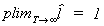

THEOREM
The LIML estimator minimizes the correlation coefficient between and Wb_j^*

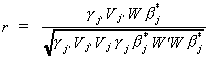
where V_j = Y_j - X_j(X_j'X_j)^-1X_j'Y_j is the residual from the regression of Y_j on the included exogenous variables and W = X_j^*-X_j(X_j'X_j)^-1X_j'X_j^* is the residual from the regression of the excluded exogenous variables on those which are included. r is known as the cannonical correlation coefficient, so LIML is also known as the minimum correlation coefficient estimator.

6.3.1.4 k-Class Estimators
Consider first the 2SLS estimator

Which we can rewrite as

If we had applied OLS to the model we would get

If we construct an estimator

then one can see that when k=0 we get OLS and when k=1 we get 2SLS.
THEOREM
Recall that we had previously said that LIML was the minimum variance ratio estimator

If we let k = in our k-class estimator then we get the LIML.
Proof:
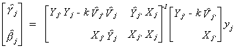
Recall
76 (1)

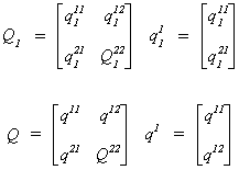
To solve for we will partition Q₁ and Q as Q₁ = [q₁¹ Q₁²] and
Q = [q¹ Q²], where q₁¹ and q¹ each have one column corresponding to the endogenous variable on the left hand side of the structural equation, and Q₁² and Q² each have the remaining m_j columns for the other included endogenous variables of the equation. This allows us to rewrite (1) as

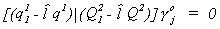
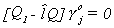
There are m_j + 1 equations in this system; we have one too many so need to discard one. We can partition further as

Given our definition 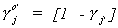, we can use our partitioning to disregard the first equation in the determinantal equation and use

Rearranging, we can derive the LIML estimator

Now suppose that there are no included exogenous variables. That is, k_j = 0 so

Note that we have Xj* in both Q22 and q21 because there is no difference between the set of all exogenous variables and the set of all excluded exogenous variables for this particular example. Substituting into we get

We conclude then that the LIML estimator is also a k class estimator.
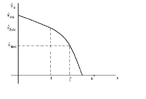
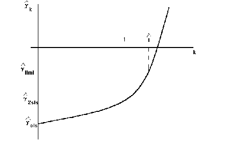
There is a problem with the k-class estimator

for some value of k the inverse explodes, so we get the follwoing relationship between the different estimators. We know that the k for LIML is always greater than 1. Therefore, the diagrams show us the ordering for the estimates, always!

6.3.2 System Methods
6.3.2.1 Three Stage Least Squares

The first equation of the structural model is

Or, using the notation we adopted for our explorations of 2SLS

In general we can write the j^th equation in the system as

Now we will put the equations together as we did for SURE. Toward that end define the following vectors and matrices

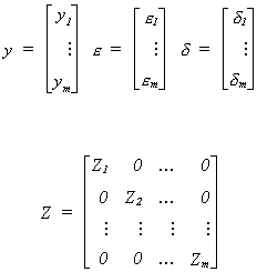
So the whole system can be written as
5 (1)

Premultiply (1) by , where X' is the kxT matrix of all observations on all of the exogenous variables.

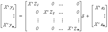7 (2)

Rewrite (2) as
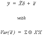8 (3)

Estimate the coefficients of (3) by GLS
9 (4)

Estimate S as follows
10 (5)

where is the 2SLS estimate. Substitute (5) into (4) to get the 3SLS estimate.

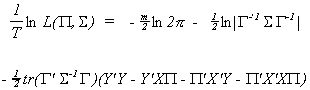
6.3.2.2 Full Information Maximum Likelihood The complete system of m structural equations is written

Using all of the observations

where the subscripts show the dimensions of the matrices. The likelihood function is . Using a theorem form distribution theory we can rewrite the likelihood as
The term at the right end of the expression is the absolute value of the determinant of the matrix of partial derivatives. You wil recognize this as the Jacobean of the transformation. In this instance it is given by so the likelihood is

Substituting in for the normal density

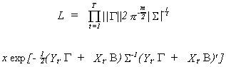
As usual it is easier to work with the log likelihood. We will also make use of the fact that the exponent is a scalar. As such, taking its trace has no effect.

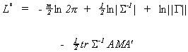
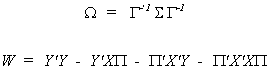
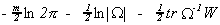
where

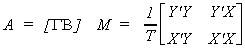
We have the following factoids from linear algebra

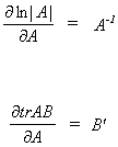
First consider

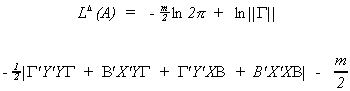
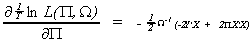
Substituting back into L^* gives us the concentrated likelihood function. The likelihood function is concentrated in the sense that we have found a maximum in the G(G+1)/2 hyperplane of the covariance parameter space.

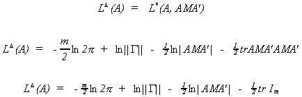
The result of substituting back in for AMA' gives

One would proceed by differentiating this with respect to the unknown coefficients, setting those partials to zero and solving. Needless to say, the first order conditions would be highly nonlinear. For years this was the stopping place in Full Information Maximum Likelihood. With the advent of cheap computing power, it became possible to write hill climbing algorithms based on the Gauss Newton principle that could solve these equations numerically. That is, in fact, how LIMDEP, RATS and TSP do their maximum likelihood estimation.
Before moving on, it is worth considering the exactly identified case. Go back to the original likelihood and substitute in the reduced form 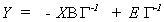to get

Define

and write the likelihood function as

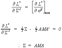
The first order condition for the maximum is

From the FOCs we can derive estimates of the reduced form parameters . Therefore, we conclude that in the exactly identified case, OLS provides us with the maximum likelihood estimates of the reduced form parameters. We could then solve the reduced form parameter equations for the structural parameter estimates.
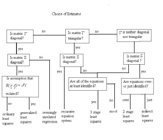
To picture the relationship between estimators I have provided the following flowchart.