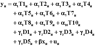
Least Squares Dummy Variables Models
Model
Specification
RSS
Log Likelihood
1
![]()
5465
-188.3
2

4827
-185.2
3

3380
-176.3
4

2663
-170.3
Random Effects - - Fixed Effects Example:
Summary
|
Least Squares Dummy Variables Models |
|||
|
Model |
Specification |
RSS |
Log Likelihood |
|
1 |
|
5465 |
-188.3 |
|
2 |
|
4827 |
-185.2 |
|
3 |
|
3380 |
-176.3 |
|
4 |
|
2663 |
-170.3 |
![]()
|
F-test Between LSDV Models |
|||
|
|
2 |
3 |
4 |
|
1 |
1.45 |
2.67 |
2.83 |
|
2 |
|
|
3.16 |
|
3 |
|
|
2.35 |
![]()
|
Random Effects Models: Chi-square Tests |
||||
|
Model |
Specification |
Estimates of Variance Components |
LM for Model j versus Model 1 |
Hausman for Model j versus Model j-3 |
|
5 |
|
|
.063 |
1.19 |
|
6 |
|
|
4.43 |
1.24 |
|
7 |
|
|
4.49 |
2.91 |
![]()
On the basis of the LM Test:
We prefer model 1 to model 5: The random individual effect is zero.
We prefer model 6 to model 1: The random time effect is not zero.
We prefer model 1 to model 7: We cannot reject the null hypothesis that both the random individual and time effects are zero.
The only REM preferred to OLS is model 6. OLS is better than either of the remaining two specifications.
On the basis of the Hausman Test:
We prefer model 5 to model 2: The random individual effect model is better than the individual fixed effect model.
We prefer model 6 to model 3: The random time effects model is better than fixed time effects model.
We prefer model 7 to model 4: The random effects model is better.
When given a choice, we never pick the fixed effects model.
![]()
CONCLUSION
From the three groups of tests we have the following intransitivity involving model 7:

so we'll eliminate 7 from the competition. From the different sets of tests we can establish the following ordering;
![]()
So we'll choose model 6 as the best model.
Home